9 Model Specification and Model Identification
9.1 From theory to model
Structural equation modelling is a confirmatory technique, i.e., we specify a model that we believe to be true in the population and test whether the specified model fits the data that we have obtained. In principle, the hypothesized model that will be fitted to the data is formulated before the data are collected. Following the stages of the in the empirical cycle as formulated by A. D. de Groot (1961), one starts with observation (the researcher observes something that deserves investigation, for example, that perfectionistic parents often have anxious children), followed by induction (reflection on, or formulation of, theories that may explain the observed phenomena), followed by deduction (the formulation of testable research hypotheses that would be implied by theory, for example, that perfectionism of parents leads to over-controlling parenting behaviour, which in turn leads to anxiety in their children). The next stage is testing the hypothesis using data. This is the phase in which the structural model that represents the research hypotheses is tested against reality (i.e., data). The last phase is evaluation, which may possibly lead to new hypotheses or revision of the theory.
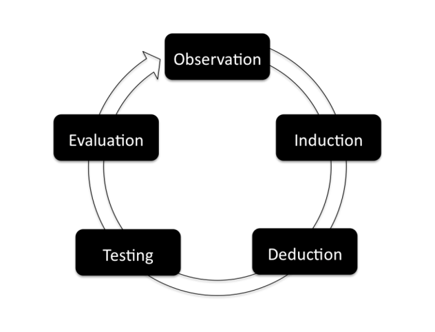
Figure 9.1: Empirical Cycle.
If there are competing theories, that each postulate a different model based on the same variables, researchers may use SEM to test the models corresponding to the different theories and select the model that fits the data best.
9.2 Model parsimony
As a researcher, you want to end up with a model that is “simple,” but that is still a good reflection of reality. In SEM, one indication of the simplicity or parsimony of a model is the degrees of freedom. For a given number of observed variables, the more degrees of freedom a model has, the more parsimonious the model (i.e., the less parameters it has, and thus the less complex the model). However, complex models with more parameters generally fit the data better. Unfortunately, this is not necessarily because the model is a more accurate description of reality; rather, freeing parameters in a data-driven way often leads to a model that is fit to sample-specific nuances. Finding the balance between parsimony and accuracy is a difficult issue. A famous principle that refers to this issue is Ockham’s razor, or the “law of parsimony” which Albert Einstein translated into the advice: “Everything should be kept as simple as possible, but no simpler”.
9.3 A priori model specification
Very often, researchers plan to fit several models. For example, if the goal is to test a mediation hypothesis, one may first fit a model with an indirect effect only, and subsequently add the direct effect to test partial mediation. Or in a full SEM model, it is common to use “two-step modeling”, which means that one first tests the measurement model, without imposing a structure on the correlations between latent variables. Only if the measurement model is accepted, one continues with specifying a path model or factor model on the latent variables. Sometimes, the hypotheses that the researchers want to tests aren’t only about the overall fit of the model, but about specific parameters in a model. For example, researchers may want to test whether certain parameters in the model are equal. This can be tested by fitting a model with and without equality constraints on these parameters, and investigate whether the fit of the model with the equality constraint is significantly worse than the fit of the model without the constraint. As long as the models that will be fitted, and the hypotheses that will be answered by these models, are formulated before looking at the data, this practice can still be called confirmatory. This is not the case if the model modifications are purely based on statistics, as will be described next.
9.4 Post hoc model modification
Often, researchers just test one theoretical model. When the model does not fit the data well, we might need to reject the notion that the model (i.e., the theory) is a true reflection of reality. When this model does not fit the data well, the model is usually modified in order to obtain better model fit. The process of sequential model modification is also called a specification search. As post-hoc model modifications (modifications to the model based on information obtained after fitting the model to the data) are inherently data-driven, they are exploratory by nature. They should be executed with great care, as they often do not lead to a model that generalizes to other samples (MacCallum, 1986). To reduce the risk of ending up with a completely sample-specific model, the specification search should always be guided by theoretically meaningful modifications. Additional strategies to reduce the risk of meaningless data-driven model modifications are to formulate a pre-specified set of parameters that are candidates for modification, to fit the model on data from large samples, and formulate the initial model very carefully. Post-hoc model modification is a data-based approach, so any final model should be evaluated as stemming from an exploratory analysis strategy, which needs to be validated in other samples. It is also important to realize that by adding parameters to the model, the discrepancies between \(\mathbf{\Sigma}_{\text{population}}\) and \(\mathbf\Sigma_{\text{model}}\) will decrease, and thus the \(χ^2\) value will become closer to zero. However, models with more parameters are also more complex and can lead to unnecessary parameters that take on meaningless values. We should strive for models that are parsimonious and can be clearly understood. So, both with the originally hypothesized model and with modified models, one needs to balance trying to find a simple and interpretable model, and arriving at good model fit.
9.5 Backward and forward specification searches
When altering a model post-hoc, there are basically two different strategies, and these strategies should not be mixed. The backward specification search involves fitting a model with many parameters, more than expected based on the theory, and then removing parameters one by one if they are not considered statistically significant. This is also called model trimming. The more popular strategy is the forward specification search, called model building. With model building one starts with a parsimonious model that only includes the parameters that are expected by theory, and add parameters when the model does not fit. The researcher can get information about which parameters will likely improve the fit of a model by inspection of correlation residuals or modification indices.
If a model doesn’t fit the data, it means that the model isn’t explaining the variances and covariances of the variables well; that is, the discrepancy between \(\hat{\mathbf{\Sigma}}_{\text{population}}\) and \(\hat{\mathbf\Sigma}_{\text{model}}\) is substantial according to the fit criteria. It may be that all covariances are very different, but it could also be that the model appropriately models the relations between some variables, but doesn’t sufficiently account for the covariances between other variables. In this case, adding parameters specifically to model the unexplained covariance may be sensible. Correlation residuals and modification indices can be used to find out from which part of the model the largest misfit arises.
9.6 Correlation residuals
Covariance residuals are the differences between the observed and model-implied covariances. That is, the matrix of covariance residuals equals the matrix of observed sample variances and covariances minus the estimated model implied matrix of variances and covariances (i.e., \(\mathbfΣ_{\text{sample}} - \hat{\mathbf\Sigma}_{\text{model}}\)). Covariance residuals have no common scale, which makes them difficult to interpret. Therefore, it may be helpful to consider the correlation residuals instead. Correlation residuals are calculated by standardizing the observed and model-implied covariance matrices, then subtracting the model-implied from the sample correlation matrix (i.e., \(\mathbfΣ^*_{\text{sample}} - \hat{\mathbf\Sigma}^*_{\text{model}}\)). Table 1 shows the correlation residuals for the full mediation model of child anxiety (i.e., the model without direct effects of Parent Anxiety and Parent Perfectionism on Child Anxiety). It can be seen that some correlations are fully explained by the model, leading to a correlation residual of zero. The correlation residual between Parental Anxiety and Child Anxiety is the largest. If a correlation residual for two variables is large, there is unmodeled dependency. As a general rule of thumb, correlation residuals with an absolute value larger than .10 are often regarded as being large. Thus, the correlation residual between Parent Anxiety and Child Anxiety lies outside the cut-off value of .10 and therefore can be considered large. Now, the researchers has to think about which parameter could be added to explain the dependency between these variables better. Here, one can choose between a direct effect or a covariance. If there are no clear ideas about the directionality of the effect, adding a covariance may be the best option. In the current example, a direct effect of PA on CA seems to make the most sense, as we already included an indirect effect of PA on CA in the model. Adding a direct effect would mean that the effect of PA and CA is not fully, but partially mediated by over-control. If a parameter is added to the model, the correlation residuals will change. Therefore, one should recalculate the correlation residuals after each model modification.
Table 1. Correlation residuals for the full mediation model of child anxiety model
| Parental Anxiety | Perfectionism | Overcontrol | Child Anxiety | |
|---|---|---|---|---|
| Parental Anxiety | .000 | |||
| Perfectionism | .000 | .000 | ||
| Overcontrol | .000 | .000 | .000 | |
| Child Anxiety | .272 | .034 | .000 | .000 |
9.7 Modification indices
Another option to investigate which possible modifications to the model could improve model fit is to look at so-called Modification Indices (MIs). MIs provide a rough estimate of how much the \(χ^2\) test statistic of a model would decrease if a particular fixed (or constrained) parameter were freely estimated. The size of a MI can be evaluated relative to a \(χ^2\) distribution with 1 \(df\). So, with a significance level of .05, one could call a MI larger than 3.84 significant. To control the inflation of Type I error rates due to multiple testing, it is recommended to (a) plan a priori which parameters’ modification indices you will inspect and (b) use a Bonferroni adjusted \(α\) level to select your critical value. For instance, the full mediation model for child anxiety only has df = 2, so you should choose no more than two modification indices to inspect. A Bonferroni-adjusted \(α = .05 / 2 = .025\) would yield a \(χ^2\) critical value of 5.02 (for a 1-\(df\) test). This is analogous to using a post hoc method (e.g., Tukey, Bonferroni, or Scheffé) to compare pairs of group means following a significant omnibus \(F\) test in ANOVA.
MIs depend on sample size. The larger the sample, the larger the modification indices. So, with large sample sizes, small misfit may already lead to large MIs. Therefore, it is useful to inspect the expected parameter change (EPC) as well. The EPC gives an indication of how a specific parameter would change if it were freely estimated. If a MI is high, but the EPC is very low, addition of the parameter would not add much to the model substantively. In addition, to enable comparison of EPCs it is often convenient to inspect the standardized version of the EPC (SEPC), where values larger than .10 are considered to be substantial (Saris & Stronkhorst, 1984). Note that MIs are univariate indices. As soon as parameter is added to (or removed from) the model, all MIs might change. Therefore, one should inspect MIs after each model modification.
Table 2 shows the MIs and SEPCs for the full mediation model of child anxiety. As you can see, the MIs are given for every parameter that is not in the model, even for parameters that do not really make sense or are mathematically not possible to add. For example, you see a MI for the direct effect of Child Anxiety on Overcontrol, as well as a covariance between these two variables. It would be strange to add one of these parameters to the model, because we already specified a direct effect from Overcontrol on Child Anxiety. Both in terms of interpretation and in terms of estimation (i.e., the model would become nonrecursive), it would be difficult to add these parameters to the model. So, as a researcher, you have to make sure to evaluate the appropriateness of parameters to be added. In the current example, the highest MI is for a covariance between CA and PA, while the MI of a direct effect of PA on CA is very similar. This is because freeing either one of these parameters would lead to an equivalent model (not equivalent in interpretation, but statistically equivalent because both models would result in the same model-implied covariance matrix). Theoretically, it makes more sense to assume that Parental Anxiety affects Child Anxiety than the other way around. Therefore, a direct effect of PA on CA seems to be the most sensible parameter to add.
Table 2. Modification indices for the full mediation model of child anxiety.
| Parameter | MI | SEPC | |
|---|---|---|---|
| Covariance: | child_anx \(↔\) parent_anx | 6.871 | .264 |
| Direct effect: | child_anx \(\leftarrow\) parent_anx | 6.716 | .292 |
| Direct effect: | parent_anx \(\leftarrow\) child_anx | 6.871 | .290 |
| Direct effect: | overcontrol \(\leftarrow\) child_anx | 2.076 | −.459 |
| Covariance: | child_anx \(↔\) overcontrol | 2.076 | −.418 |
| Direct effect: | perfectionism \(\leftarrow\) child_anx | .598 | −.087 |
| Direct effect: | child_anx \(\leftarrow\) perfectionism | .109 | .038 |
| Covariance: | perfectionism \(↔\) child_anx | .598 | −.079 |
The lavaan Script 9.0 below demonstrates how to make a minor model adjustment, such as adding a single parameter. Note that the model syntax does not need to be a single character string, but can be a vector of character strings, so we do not need to write out the whole model again. The new model can be fit to the data using all the same lavaan() arguments in Script 3.1, or we can use the update() function as a shortcut. Any specified arguments will replace the original model-fit arguments found in the object AWmodelOut. The first argument to lavaan() is called model), so we provide our new model syntax. All other (unspecified) arguments will be the same when the new model is fit, saving the results in the object AWmodel2Out.
9.7.1 Script 9.0
# add a direct effect of Parent Anxiety on Child Anxiety to the path model
AWmodel2 <- c(AWmodel, ' child_anx ~ b41* parent_anx ')
# fit the new model by "updating" the original model
AWmodel2Out <- update(AWmodelOut, model = AWmodel2)
## Warning: lavaan->ldw_parse_model_string():
## modifier label specified multiple times, overwritten at line 25, pos 14
## child_anx ~ b41* parent_anx
## ^In our illustrative example of child anxiety, the partial mediation model (where the regression of child anxiety on parent anxiety is added to the model) yields the following test result: \(χ^2(1) = 0.397\), \(p = .53\). Thus, the \(χ^2\) value is no longer significant (at \(α = .05\)), so the null hypothesis of exact fit cannot be rejected. This gives support to the notion that the model gives a true description of reality. However, one could question the parsimony of this model with a single degree of freedom. The size of the direct effect in standardized metric is estimated to be .292, which is substantial. Note that the actual value matches the SEPC in Table 2 to the third decimal place. Expected and actual estimated values will not always correspond so perfectly, but they will typically be very close.
9.8 Cross-validation
When post hoc model modification is used, one is actually not testing hypotheses anymore, but one is generating hypotheses based on the data under consideration. That is, it falls under exploratory research, and its results carry less scientific certainty than the results of confirmatory research. Future research could focus on trying to replicate the findings based on the final model from exploratory research.
9.9 Calculating correlation residuals in lavaan
The residual() function (or resid() for short) provides covariance residuals by default, but you can request correlation residuals with an additional argument:
## $type
## [1] "cor.bollen"
##
## $cov
##             ovrcnt chld_n prnt_n perfct
## overcontrol  0.000
## child_anx    0.000  0.000
## parent_anx   0.000  0.272  0.000
## perfect      0.000  0.034  0.000  0.000
## the default standardization method is Bollen's (1989) formula
resid(AWmodelOut, type = "cor.bollen")## $type
## [1] "cor.bollen"
##
## $cov
## ovrcnt chld_n prnt_n perfct
## overcontrol 0.000
## child_anx 0.000 0.000
## parent_anx 0.000 0.272 0.000
## perfect 0.000 0.034 0.000 0.000## optionally, arrange rows & columns to match input order
resid(AWmodelOut, type = "cor")$cor[obsnames, obsnames]## NULLFirst, we created two objects that contain the sample (ssam) and model-implied (smod) covariance matrices. Although the sample covariance matrix is available as the object AWcov that was used as input data, this would not be the case if raw data were analysed. And although we could calculate the sample covariance matrix for complete data using the cov() function, when there are missing data, covariance and correlation residuals must be calculated using the estimated covariance matrix (also called the EM matrix) that is obtained by fitting the saturated model to the partially observed data. Thus, the most error-free way to extract this information from lavaan is to use the lavInspect() function to extract the sample statistics, or “sampstat” for short. Likewise, the model-implied covariance matrix can be extracted by requesting “cov.ov” (i.e., the model-implied covariance between observed variables).
# extract the sample covariance matrix
ssam <- lavInspect(AWmodelOut, "sampstat")$cov
# extract the model-implied covariance matrix
smod <- lavInspect(AWmodelOut, "cov.ov")
These matrices need to be standardized. This is done with the R function cov2cor(), which transforms a covariance matrix to a correlation matrix. The model-implied correlation matrix is then subtracted from the observed correlation matrix, and we print the result rounded to the third decimal place:
##             ovrcnt chld_n prnt_n perfct
## overcontrol  0.000
## child_anx    0.000  0.000
## parent_anx   0.000  0.272  0.000
## perfect      0.000  0.034  0.000  0.000
The last two lines are optional, but may help you find the large (> .10) and largest residuals, respectively, indicated by cells saying TRUE.
##             overcontrol child_anx parent_anx perfect
## overcontrol       FALSE     FALSE      FALSE   FALSE
## child_anx         FALSE     FALSE       TRUE   FALSE
## parent_anx        FALSE      TRUE      FALSE   FALSE
## perfect FALSE FALSE FALSE FALSE## overcontrol child_anx parent_anx perfect
## overcontrol FALSE FALSE FALSE FALSE
## child_anx FALSE FALSE TRUE FALSE
## parent_anx FALSE TRUE FALSE FALSE
## perfect FALSE FALSE FALSE FALSENote that there is also a slightly different formula available, which is implemented in Bentler’s (1995) EQS software. Rather than standardizing each matrix with respect to their own \(SD\)s, then subtracting them, Bentler proposed subtracting the unstandardized covariance matrices, then standardizing the differences with respect to the observed-variable \(SD\)s only. Script 8.2 shows how to request these correlation residuals from lavaan, as well as how the procedure to calculate them differs.
##             ovrcnt chld_n prnt_n perfct
## overcontrol  0.000
## child_anx    0.000  0.000
## parent_anx   0.000  0.272  0.000
## perfect      0.000  0.034  0.000  0.000
## MANUAL PROCEDURE:
## calculate covariance residuals
covres <- ssam - smod
## standardize covariance residuals to make correlation residuals
SDs <- diag(sqrt(diag(ssam)))
dimnames(SDs) <- dimnames(covres)
corres <- solve(SDs) %*% covres %*% solve(SDs)
round(corres, 3)## overcontrol child_anx parent_anx perfect
## overcontrol 0 0.000 0.000 0.000
## child_anx 0 0.000 0.272 0.034
## parent_anx 0 0.272 0.000 0.000
## perfect 0 0.034 0.000 0.000n this case, you will not notice any difference between the two procedures. The reason is that when no constraints are placed on the (residual) variance estimates, the estimated values will be chosen such that the model-implied total variance will exactly reproduce the observed total variance. In such situations, there is no practical difference between the two formulae.
In situations where the variances are constrained (see, for example, later chapters on strict measurement invariance), the two formulae will diverge, and neither is “right” or “wrong” because they are both standardized, but with respect to different criteria. Because Bollen’s (1989) formula standardizes the observed and model-implied matrices first, the diagonals will always be 1 by definition, so diagonal elements of the correlation-residual matrix will always be \(1 – 1 = 0\). Bentler’s (1995) formula, on the other hand, might be more helpful to identify invalid constraints on (residual) variances because the differences between observed and model-implied variances are calculated first, then standardized with respect to how large the “true” observed variances are.
9.9.1 Requesting MIs and (S)EPCs in lavaan
In lavaan, MIs and EPCs can be inspected using the modificationIndices() function. This function returns a data frame with the complete list of model parameters that are fixed to a specific value (i.e., not for equality constraints), and prints each associated MI and (standardized and unstandardized) EPC. Using the following commands, the data frame is sorted with the highest MIs printed first. Also, we can specify a minimum value (i.e., a critical value, crit) to display only MIs that might be considered significant. Here, we define it as a \(1-df\) \(χ^2\) value corresponding to \(α = .05\):
crit <- qchisq(.05, df = 1, lower.tail = FALSE)
modificationIndices(AWmodelOut, sort. = TRUE, minimum.value = crit)
The output for all nonzero MIs from the model are given below.
          lhs op        rhs    mi   epc sepc.lv sepc.all sepc.nox
12  child_anx ~~ parent_anx 6.871 6.945   6.945    0.264    0.264
18 parent_anx  ~  child_anx 6.871 1.009   1.009    0.290    0.290
15  child_anx  ~ parent_anx 6.716 0.084   0.084    0.292    0.292
You can also request that MIs be printed at the bottom of the summary() output, but you have no options to sort or subset them:
References
Bentler, P. M. (1995). EQS structural equations program manual. Encino, CA: Multivariate Software.
Bollen, K. A. (1989). Structural equations with latent variables. Hoboken, NJ: Wiley.
MacCallum, R. C. (1986). Specification searches in covariance structure modelling. Psychological Bulletin, 100(1), 107–120. doi:10.1037/0033-2909.100.1.107
Saris, W. E., & Stronkhorst, H. (1984). Causal modelling in nonexperimental research: An introduction to the LISREL approach. Amsterdam, NL: Sociometric Research Foundation.