17 Second Order Factor Models
The expression for a factor model is \(\mathbfΣ_{\text{model}} = \mathbfΛ \mathbfΦ \mathbfΛ’+ \mathbfΘ\). In a hierarchical factor model, the covariances between the common factors in \(\mathbfΦ\) are modeled by a second-order factor model, \(\mathbfΦ = \mathbfΛ_2 \mathbfΦ_2 \mathbfΛ_2’+ \mathbfΘ_2\), where \(\mathbfΦ\) denotes the covariances between first-order factors, \(\mathbfΛ_2\) is a full matrix with second-order factor loadings, \(\mathbfΦ_2\) is a symmetric matrix with variances and covariances of the second-order factors and \(\mathbfΘ_2\) is a diagonal matrix with the variances of the second-order residual factors.
Script 17.1 fits a second order factor model to the data of the School Attitudes Questionnaire (SAQ; Smits & Vorst, 1982) from Chapter 14. Instead of having all three latent variables correlate with each other, we hypothesize that there is one second-order common factor (Attitudes) that explains the correlations between the first-order common factors. This model is depicted in Figure 17.1.
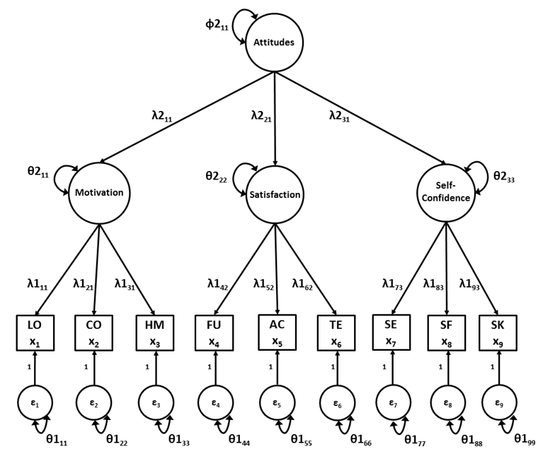
Figure 17.1: Second-order factor model for the School Attitudes Questionnaire
Script 17.1
## Specify second-order factor model
saqmodel2nd <- '
    # FIRST-ORDER PART
    # factor loadings
    Motivation =~ L11*learning + L21*concentration + L31*homework
    Satisfaction =~ L42*fun + L52*acceptance + L62*teacher
    SelfConfidence =~ L73*selfexpr + L83*selfeff + L93*socialskill

    # residual variances observed variables
    learning ~~ TH11*learning
    concentration ~~ TH22*concentration
    homework ~~ TH33*homework
    fun ~~ TH44*fun
    acceptance ~~ TH55*acceptance
    teacher ~~ TH66*teacher
    selfexpr ~~ TH77*selfexpr
    selfeff ~~ TH88*selfeff
    socialskill ~~ TH99*socialskill

    # scaling constraints
    L11 == 1
    L42 == 1
    L73 == 1

    # SECOND-ORDER PART
    # factor loadings second-order
    Attitudes =~ L11_2*Motivation + L21_2*Satisfaction +
                   L31_2*SelfConfidence

    # residual variances first-order common factors
    Motivation ~~ TH11_2*Motivation
    Satisfaction ~~ TH22_2*Satisfaction
    SelfConfidence ~~ TH33_2*SelfConfidence

    # variance second-order common factor
    Attitudes ~~ F11_2*Attitudes

    # scaling constraints
    L11_2 == 1
'

## Run model
saqmodel2ndOut <- lavaan(saqmodel2nd, sample.cov = saqcov,
                         sample.nobs = 915, likelihood = "wishart",
                         fixed.x = FALSE)
## Output
summary(saqmodel2ndOut, fit = TRUE, std = TRUE)
So, in the first part of the script, we create the “First-order part” of the model. We specify the parameters of the \(\mathbfΛ\) matrix (factor loadings) and Θ matrix (residual variances observed indicators), but do not specify the parameters of the Φ matrix (the variances and covariances of the first-order common factors) as this matrix is now a function of second-order factor loadings (\(\mathbfΛ_2\)), second-order factor variances and covariances (\(\mathbfΦ_2\)) and second-order residual variances and covariances (\(\mathbfΘ_2\)).
In second-order factor analysis, it is difficult to scale the first-order factors by fixing their variances to 1, because the \(\mathbfΦ\) matrix is not directly defined. Therefore we scaled the first-order common factors by fixing the first factor loading of each factor to 1. Scaling of the second-order factors can be done through factor loadings or factor variances. In the current example we scaled the second-order factor through one of the factor loadings.
The “Second-order part” of the model thus consists of the regression equations that define the second-order factor, the residual variances of the three first-order common factors, and the variance of the second-order common factor:
    # regression equations
    Attitudes =~ L11_2*Motivation + L21_2*Satisfaction +
                   L31_2*SelfConfidence

    # residual variances first-order common factors
    Motivation ~~ TH11_2*Motivation
    Satisfaction ~~ TH22_2*Satisfaction
    SelfConfidence ~~ TH33_2*SelfConfidence

    # variance second-order common factor
    Attitudes ~~ F11_2*Attitudes
We have used similar labels as we have used for the first-order part of the model, but added “_2” to the labels to distinguish them.
Finally, we run the model using the lavaan() function and request the output using the summary() function. The output consists of two parts: “Latent variables” and “Variances”. In the presentation of the output lavaan does not distinguish between first order and second order parameter estimates.
Notice that the estimated residual variance of the first order factor Motivation is negative, representing a so-called “Heywood case” or inadmissible solution. A Heywood case is a sign of either (a) model misspecification or (b) sampling error. When a true parameter is close to a boundary (e.g., small residual variances, high correlations or standardized loadings) and our sample is not asymptotically large, non-problematic Heywood cases are actually quite common. A better solution is to directly investigate the apparent problem by checking both (a) and (b) to see whether is a sufficient explanation of the Heywood case.
*We check (a) using \(χ^2\), or by using approximate fit measures to see if the misfit is severe enough to suggest a bad model.
*We check (b) by looking at the 95% CI or Wald \(z\) statistic for the Heywood case. If we can’t reject the null hypothesis that the true parameter is a plausible value, AND our model does not appear to be terribly misspecified, then we can’t dismiss sampling error as the cause.
In this example, the estimated variance is −1.675, but the \(SE = 1.704\), so the CI includes positive values. RMSEA indicates mediocre fit, and \(\text{CFI} > .95\), so it would be reasonable to conclude that the 2nd-order factor explains most variance in Motivation, and that the estimate is negative only because of sampling error.
Getting the parameter estimates in matrix form
The lavaan package uses a slightly different parameterization of structural equation models than we do. All unidirectional effects between latent variables are part of matrix beta, and all (residual) variances and covariances of latent variables are part of matrix psi in lavaan. So, the second-order factor loadings, \(\mathbfΛ_2\), are part of matrix beta, and the second-order factor variances and covariances, \(\mathbfΦ_2\), as well as the second-order residual variances of the second order model, \(\mathbfΘ_2\), are part of matrix psi. You can extract the parameter estimates in matrix form using the names of the variables and factors with the following code:
Script 17.2
Estimates <- lavInspect(saqmodel2ndOut, "est")

factor1names <- c("Motivation","Satisfaction","SelfConfidence")
factor2names <- c("Attitudes")

lambda1 <- Estimates$lambda[obsnames, factor1names]
theta1 <- Estimates$theta[obsnames, obsnames]
lambda2 <- Estimates$beta[factor1names, factor2names, drop = FALSE]
theta2 <- Estimates$psi[factor1names, factor1names]
phi2 <- Estimates$psi[factor2names, factor2names, drop = FALSE]

phi1 <- lambda2 %*% phi2 %*% t(lambda2) + theta2
That is, by selecting the appropriate rows and columns using the names of the observed variables, first order common factors, and second order common factors, one can extract the submatrices from the larger matrices that lavaan uses. For psi2 and lambda2, we used the drop = FALSE argument in this example. This is only necessary if lambda2 has only 1 column (i.e. if there is a single second-order factor). When extracting more than 1 column (and row) from a matrix, the result will remain a matrix automatically.
Notice that the phi1 matrix is now calculated using \(\mathbfΦ_1 = \mathbfΛ_2 \mathbfΦ_2 \mathbfΛ_2’+ \mathbfΘ_2\), because in the second-order factor model the variances and covariances of the first-order common factors are modelled as a function of second-order parameters.
17.1 Standardized parameter estimates for the higher-order part of the model
In addition to obtaining standardized estimates for (first-order) factor loadings and residual variances (as described in Chapter 13), we can also obtain standardized estimates for the second-order factor loadings, residual variances, and second-order common factor variances and covariances using matrix algebra.
Standardization of the second-order coefficients involves calculating the parameter estimates that would be obtained if the standard deviations of all first- and second-order factors were equal to 1.
Script 17.3 has commands that can be added to Script 17.2 to calculate the standardized parameters of the second order part of the model.
Script 17.3
## calculate standard deviations first- and second-order common factors
SDphi1 <- diag(sqrt(diag(phi1)))
SDphi2 <- diag(sqrt(diag(phi2)), nrow = 1, ncol = 1)

## calculate standardized parameters
lambda2star <- solve(SDphi1) %*% lambda2 %*% SDphi2
phi2star <- solve(SDphi2) %*% phi2 %*% solve(SDphi2)
theta2star <- solve(SDphi1) %*% theta2 %*% solve(SDphi1)
struc2 <- lambda2star %*% phi2star

## give labels to matrices
dimnames(lambda2star) <- list(factor1names, factor2names)
dimnames(phi2star) <- list(factor2names, factor2names)
dimnames(theta2star) <- list(factor1names, factor1names)
dimnames(struc2) <- list(factor1names, factor2names)
The operations that are used to calculate the standardized parameters of the second-order part of the hierarchical factor model are identical to standardization of the first-order part of a factor model. The difference is that we now extract the parameter estimates of the second-order part of the model, and we use the standard deviations of the first-order common factors (instead of the observed indicators) and the standard deviations of the second-order common factors (instead of the first-order common factors).
Notice that we used the nrow and ncol arguments to the outer diag() function when creating SDphi2. Recall that the inner call to diag() is used to extract the diagonal of phi2. The outer call to diag() is used to create a matrix. There are actually two ways that diag() will accept your instructions:
-If you give it a vector of numbers, it will place those numbers on the diagonal. So the dimensions of the resulting matrix will be determined by how many numbers are in the vector. For example, sqrt(diag(phi1)) contains three standard deviations, so diag(sqrt(diag(phi1))) creates a \(3 × 3\) diagonal matrix.
-If you give it a single number, it will drop any decimal values and give you an identity matrix (ones on the diagonal) with that many rows and columns. For example, sqrt(diag(phi2)) contains only one standard deviation (\(SD = 3.196\)), so diag(sqrt(diag(phi2))) would create a \(3 × 3\) identity matrix. To correctly return a \(1 × 1\) matrix with 3.196 on the “diagonal,” we need to explicitly tell diag() that we want 1 row and 1 column.