26 Longitudinal Factor Analysis
With longitudinal factor analysis, a factor model is fitted to a set of indicators of which responses are collected at different time points. It may be interesting to compare factor means and variance across time.
Fitting a longitudinal factor model is not very different from fitting a factor model with means, except that in a longitudinal factor model there are covariances between the residual factors of the same indicator at different time points. Figure 1 depicts a one-factor model of “Self-efficacy” with six indicators, measured at two different time points. Because each indicator is measured twice in the same individuals, the item specific components of each indicator covary across timepoints.
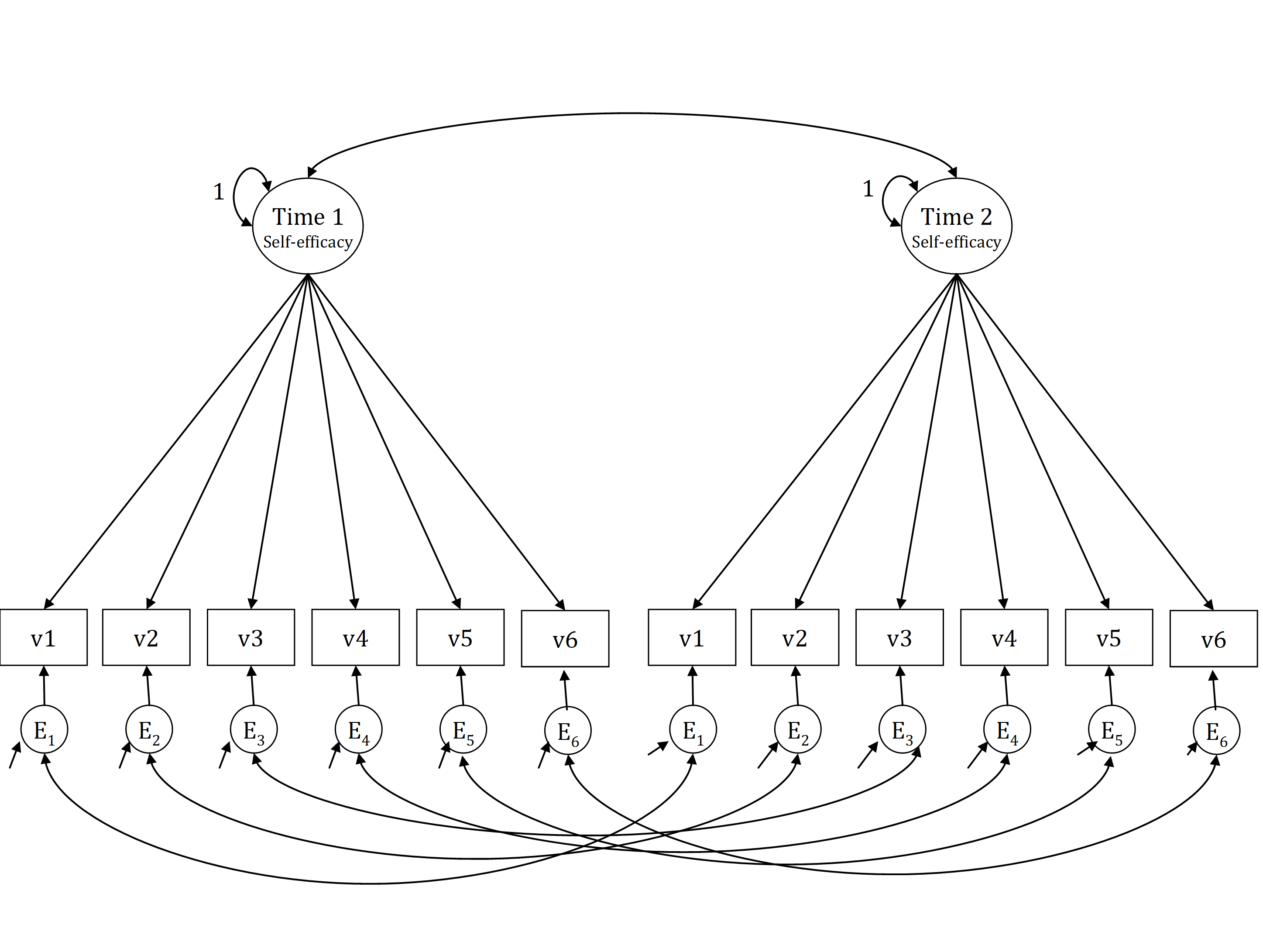
Figure 26.1: Self-efficacy measured at two time points.
In order to compare latent variances or latent means over across timepoints, the measurement of the latent variables should be equal over time. To test longitudinal invariance, we can use similar steps as when testing measurement invariance across groups:
- Configural invariance. Fit the same factor model to all time points (with residual covariances).
- Weak factorial invariance. Fit a model with equality constraints on the factor loadings across time, and free factor variances at the later time points.
- Strong factorial invariance. Fit a model with additional equality constraints on the intercepts across time, and free factor means at later time points.
- Strict factorial invariance. Fit a model with additional equality constraints on the residual factor variances across time points.
The last step (strict factorial invariance) is not required for a valid comparison of common factor means, variances, or covariances across occasions, but it is required (along with equality of common-factor variances over time) to test the assumption that the observed indicators are measured with the same reliability across time points.
26.1 Step 1: A longitudinal factor model with configural invariance
Script 26.1 fits the model from Figure 1 to data from Hornstra, van der Veen, Peetsma and Volman (2013), without equality constraints across time.
Script 26.1
## observed data

obsnames <- c("t1v1","t1v2","t1v3","t1v4","t1v5","t1v6",
         "t2v1","t2v2","t2v3","t2v4","t2v5","t2v6")

values <- c(
0.5237,
0.2387, 0.6653,
0.0606, 0.0576, 0.6169,
0.1260, 0.1640, 0.1800, 0.6467,
0.1489, 0.2452, 0.0621, 0.1665, 0.6151,
0.2383, 0.3781, 0.1109, 0.2248, 0.3143, 0.7241,
0.2691, 0.1920, 0.0778, 0.1296, 0.1445, 0.2599, 0.6678,
0.1686, 0.2949, 0.0952, 0.1548, 0.2139, 0.3171, 0.3080, 0.7102,
0.0881, 0.0667, 0.1673, 0.0872, 0.0719, 0.0852, 0.1681, 0.1604, 0.6583,
0.1473, 0.1594, 0.0795, 0.2021, 0.1393, 0.1769, 0.2639, 0.2910, 0.1445, 0.6218,
0.1744, 0.2025, 0.0899, 0.1621, 0.2381, 0.2736, 0.2792, 0.3640, 0.1411, 0.3163, 0.7072,
0.2192, 0.2630, 0.1325, 0.1730, 0.2348, 0.3630, 0.3613, 0.4471, 0.1884, 0.2894, 0.4354, 0.7768)

hornstracov <- getCov(x=values, names = obsnames)

hornstrameans <- c(3.3640, 3.4138, 3.9444, 3.8544, 3.8391, 3.1992, 3.4674, 3.4693, 4.0057, 3.9119, 3.8218, 3.2778)
names(hornstrameans) <- obsnames

## STEP 1: define longitudinal model without equality constraints
hornstramodel1 <- '
            # COVARIANCES
            # regression equations
            selfeff1 =~ t1v1 + t1v2 + t1v3 + t1v4 + t1v5 + t1v6
            selfeff2 =~ t2v1 + t2v2 + t2v3 + t2v4 + t2v5 + t2v6

            # residual variances
            t1v1 ~~ t1v1
            t1v2 ~~ t1v2
            t1v3 ~~ t1v3
            t1v4 ~~ t1v4
            t1v5 ~~ t1v5
            t1v6 ~~ t1v6
            t2v1 ~~ t2v1
            t2v2 ~~ t2v2
            t2v3 ~~ t2v3
            t2v4 ~~ t2v4
            t2v5 ~~ t2v5
            t2v6 ~~ t2v6

            # residual covariances
            t1v1 ~~ t2v1
            t1v2 ~~ t2v2
            t1v3 ~~ t2v3
            t1v4 ~~ t2v4
            t1v5 ~~ t2v5
            t1v6 ~~ t2v6

            # common factor (co)variances
            selfeff1 ~~ 1*selfeff1
            selfeff2 ~~ 1*selfeff2
            selfeff1 ~~ selfeff2

            # MEANS
            # intercepts observed indicators
            t1v1 ~ 1
            t1v2 ~ 1
            t1v3 ~ 1
            t1v4 ~ 1
            t1v5 ~ 1
            t1v6 ~ 1
            t2v1 ~ 1
            t2v2 ~ 1
            t2v3 ~ 1
            t2v4 ~ 1
            t2v5 ~ 1
            t2v6 ~ 1

            # means common factors
            selfeff1 ~ 0*1
            selfeff2 ~ 0*1
            '
## run the model
hornstramodel1Out <- lavaan(hornstramodel1, sample.cov = hornstracov,
                     sample.mean = hornstrameans, sample.nobs = 522,
               likelihood = "normal", fixed.x = FALSE)
## output
summary(hornstramodel1Out)
Actually, the longitudinal factor model is an ordinary factor model (with mean structure). Differences are present in the \(\mathbfΘ\) matrix, where we have now specified residual factor covariances between the residual factors of the same indicators across time.
26.2 Step 2: A longitudinal model with weak factorial invariance.
Script 26.2 shows how to fit the model from Figure 1 to the data of Hornstra et al. with equality constraints on the factor loadings across time, and free to be estimated factor variances at the later time points.
Script 26.2
## STEP 2
## constrain factor loadings to be equal across occasions
hornstramodel2 <- '
            # COVARIANCES
            # regression equations
            selfeff1 =~ L1*t1v1 + L2*t1v2 + L3*t1v3 + L4*t1v4 +
                              L5*t1v5 + L6*t1v6
            selfeff2 =~ L1*t2v1 + L2*t2v2 + L3*t2v3 + L4*t2v4 +
                              L5*t2v5 + L6*t2v6

            # residual variances
            t1v1 ~~ t1v1
            t1v2 ~~ t1v2
            t1v3 ~~ t1v3
            t1v4 ~~ t1v4
            t1v5 ~~ t1v5
            t1v6 ~~ t1v6
            t2v1 ~~ t2v1
            t2v2 ~~ t2v2
            t2v3 ~~ t2v3
            t2v4 ~~ t2v4
            t2v5 ~~ t2v5
            t2v6 ~~ t2v6

            # residual covariances
            t1v1 ~~ t2v1
            t1v2 ~~ t2v2
            t1v3 ~~ t2v3
            t1v4 ~~ t2v4
            t1v5 ~~ t2v5
            t1v6 ~~ t2v6

            # common factor (co)variances
            selfeff1 ~~ 1*selfeff1
            selfeff2 ~~ selfeff2
            selfeff1 ~~ selfeff2

            # MEANS
            # intercepts observed indicators
            t1v1 ~ 1
            t1v2 ~ 1
            t1v3 ~ 1
            t1v4 ~ 1
            t1v5 ~ 1
            t1v6 ~ 1
            t2v1 ~ 1
            t2v2 ~ 1
            t2v3 ~ 1
            t2v4 ~ 1
            t2v5 ~ 1
            t2v6 ~ 1

            # means common factors
            selfeff1 ~ 0*1
            selfeff2 ~ 0*1
            '

## run model
hornstramodel2Out <- lavaan(hornstramodel2, sample.cov = hornstracov,
                     sample.mean = hornstrameans, sample.nobs = 522,
               likelihood = "normal", fixed.x = FALSE)

## output
summary(hornstramodel2Out)

## compare fit with configural model
anova(hornstramodel1Out,hornstramodel2Out)
We constrain the factor loadings of the same indicator to be equal across time points, by using identical labels for the factor loadings. Because with this equality constraint the variance of the common factor of the second measurement is already identified, we can freely estimate this parameter (do not forget to release the constraint!).
The fit of this model can be compared to the model fit of the model without any across occasion constraints to test whether the equality constraints on the factor loadings lead to a (significant) deterioration in model fit. When the deterioration in fit is not significant, we may conclude that the assumption of weak factorial invariance holds.
26.3 Step 3: Longitudinal model with strong factorial invariance
Script 26.3 shows how to fit the model with additional equality constraints on the intercepts across time, and free to be estimated factor means at later time points.
Script 26.3
## STEP 3
## Constrain intercepts to be equal across occasions
hornstramodel3 <- '
            # COVARIANCES
            # regression equations
            selfeff1 =~ L1*t1v1 + L2*t1v2 + L3*t1v3 + L4*t1v4 +
                              L5*t1v5 + L6*t1v6
            selfeff2 =~ L1*t2v1 + L2*t2v2 + L3*t2v3 + L4*t2v4 +
                              L5*t2v5 + L6*t2v6

            # residual variances
            t1v1 ~~ t1v1
            t1v2 ~~ t1v2
            t1v3 ~~ t1v3
            t1v4 ~~ t1v4
            t1v5 ~~ t1v5
            t1v6 ~~ t1v6
            t2v1 ~~ t2v1
            t2v2 ~~ t2v2
            t2v3 ~~ t2v3
            t2v4 ~~ t2v4
            t2v5 ~~ t2v5
            t2v6 ~~ t2v6

            # residual covariances
            t1v1 ~~ t2v1
            t1v2 ~~ t2v2
            t1v3 ~~ t2v3
            t1v4 ~~ t2v4
            t1v5 ~~ t2v5
            t1v6 ~~ t2v6

            # common factor (co)variances
            selfeff1 ~~ 1*selfeff1
            selfeff2 ~~ selfeff2
            selfeff1 ~~ selfeff2

            # MEANS
            # intercepts observed indicators
            t1v1 ~ T1*1
            t1v2 ~ T2*1
            t1v3 ~ T3*1
            t1v4 ~ T4*1
            t1v5 ~ T5*1
            t1v6 ~ T6*1
            t2v1 ~ T1*1
            t2v2 ~ T2*1
            t2v3 ~ T3*1
            t2v4 ~ T4*1
            t2v5 ~ T5*1
            t2v6 ~ T6*1

            # means common factors
            selfeff1 ~ 0*1
            selfeff2 ~ 1
            '

## run model
hornstramodel3Out <- lavaan(hornstramodel3, sample.cov = hornstracov,
                     sample.mean = hornstrameans, sample.nobs = 522,
               likelihood = "normal", fixed.x = FALSE)

## output
summary(hornstramodel3Out)

## compare fit with weak factorial invariance model
anova(hornstramodel2Out,hornstramodel3Out)
Again, we use labels to constrain the intercepts to be equal across occasions. This allows us to freely estimate the common factor mean of self-efficacy at the second time point. To test whether the assumption of strong factorial invariance holds, we can compare the model fit of this model to the model fit of the model without equality constraints imposed on the intercepts.
26.4 Step 4: A model with strict factorial invariance
Sometimes, additional equality constraints are imposed on the residual factor variances across time. This is also referred to as ‘strict factorial invariance’. We can use labels to impose the equality constraints, similar like we did with the intercepts. Script 26.4 shows how to fit this model.
Script 26.4
## STEP 4: Additional constraints on THETA
hornstramodel4 <- '
            # COVARIANCES
            # regression equations
            selfeff1 =~ L1*t1v1 + L2*t1v2 + L3*t1v3 + L4*t1v4 +
                              L5*t1v5 + L6*t1v6
            selfeff2 =~ L1*t2v1 + L2*t2v2 + L3*t2v3 + L4*t2v4 +
                              L5*t2v5 + L6*t2v6

            # residual variances
            t1v1 ~~ TH1*t1v1
            t1v2 ~~ TH2*t1v2
            t1v3 ~~ TH3*t1v3
            t1v4 ~~ TH4*t1v4
            t1v5 ~~ TH5*t1v5
            t1v6 ~~ TH6*t1v6
            t2v1 ~~ TH1*t2v1
            t2v2 ~~ TH2*t2v2
            t2v3 ~~ TH3*t2v3
            t2v4 ~~ TH4*t2v4
            t2v5 ~~ TH5*t2v5
            t2v6 ~~ TH6*t2v6

            # residual covariances
            t1v1 ~~ t2v1
            t1v2 ~~ t2v2
            t1v3 ~~ t2v3
            t1v4 ~~ t2v4
            t1v5 ~~ t2v5
            t1v6 ~~ t2v6

            # common factor (co)variances
            selfeff1 ~~ 1*selfeff1
            selfeff2 ~~ selfeff2
            selfeff1 ~~ selfeff2

            # MEANS
            # intercepts observed indicators
            t1v1 ~ T1*1
            t1v2 ~ T2*1
            t1v3 ~ T3*1
            t1v4 ~ T4*1
            t1v5 ~ T5*1
            t1v6 ~ T6*1
            t2v1 ~ T1*1
            t2v2 ~ T2*1
            t2v3 ~ T3*1
            t2v4 ~ T4*1
            t2v5 ~ T5*1
            t2v6 ~ T6*1

            # means common factors
            selfeff1 ~ 0*1
            selfeff2 ~ 1
            '

## run model
hornstramodel4Out <- lavaan(hornstramodel4, sample.cov = hornstracov,
                     sample.mean = hornstrameans, sample.nobs = 522,
               sample.cov.rescale = FALSE, fixed.x = FALSE)

## output
summary(hornstramodel4Out)

## compare fit with strong factorial invariance model
anova(hornstramodel3Out,hornstramodel4Out)
26.5 Standardized estimates for a (longitudinal) factor model with means
Standardizing a longitudinal factor model works the same as standardizing a normal factor model, only now we also have a mean structure which can be standardized. To extract the estimates in matrix form from the lavaan output, including the estimates for the intercepts of the observed indicators and the common factor means, we use the lavInspect() function.
Script 26.5 has the code that uses matrix algebra to obtain the standardized parameter estimates.
Script 26.5
factornames <- c("selfeff1","selfeff2")
Estimates <- lavInspect(hornstramodel3Out, "est")

LAMBDA    <- Estimates$lambda[obsnames, factornames]
PHI       <- Estimates$psi[factornames, factornames]
THETA     <- Estimates$theta[obsnames, obsnames]
TAU       <- Estimates$nu[obsnames,1,drop=FALSE]
KAPPA     <- Estimates$alpha[factornames,1,drop=FALSE]

# Model implied covariance matrix (SIGMA) and mean vector (MU)
SIGMA     <- LAMBDA %*% PHI %*% t(LAMBDA) + THETA
MU      <- TAU + LAMBDA %*% KAPPA

## calculate standard deviations sigma and phi
SDSIGMA <- sqrt(diag(diag(SIGMA)))
SDPHI   <- sqrt(diag(diag(PHI)))

## calculate standardized parameters
LAMBDAstar  <- solve(SDSIGMA) %*% LAMBDA %*% SDPHI
PHIstar     <- solve(SDPHI) %*% PHI %*% solve(SDPHI)
THETAstar   <- solve(SDSIGMA) %*% THETA %*% solve(SDSIGMA)
STRUC   <- LAMBDAstar %*% PHIstar
KAPPAstar   <- KAPPA * diag(solve(SDPHI))
TAUstar     <- TAU * diag(solve(SDSIGMA))

## provide labels
dimnames(LAMBDAstar)  <- list(obsnames,factornames)
dimnames(PHIstar)     <- list(factornames,factornames)
dimnames(THETAstar)   <- list(obsnames,obsnames)
dimnames(STRUC)         <- list(obsnames,factornames)
dimnames(KAPPAstar)   <- list(factornames,"Common factor means")
dimnames(TAUstar)     <- list(obsnames,"Intercepts")
The intercepts (TAU) and factor means (KAPPA) are part of respectively the ‘mu’ (\(\mathbf\mu\)) and ‘alpha’(\(\mathbf\alpha\)) matrices in lavaan. We extract them by selecting the rows that correspond to the observed variable names for TAU and with the factor names for KAPPA. The ‘1’ specifies that we want to select the first column, and drop = FALSE is needed to ensure that the result is stored in a column vector.
TAU       <- Estimates$nu[obsnames,1,drop=FALSE]
KAPPA     <- Estimates$alpha[factornames,1,drop=FALSE]
The common factor means are standardized by multiplying the column vector with the factor means with a vector with the inverse of the factor standard deviations. As the standard deviations are on the diagonal of SDPHI, we use the diag() function to extract the diagonal elements. By using simple multiplication * (as opposed to matrix multiplication) the first elements of the two object are multiplied with each other, the second elements with each other, and so on. Intercepts are standardized in the same way as factor means, but with respect to the standard deviations of the observed variables:
KAPPAstar   <- KAPPA * diag(solve(SDPHI))
TAUstar     <- TAU * diag(solve(SDSIGMA))
Alternatively, you can specify “standardized = TRUE” in the summary() function.