13 Fitting Path Models with Multilevel Data
Research in the field of child development or education often involves nested observations. For example, data may be gathered by first selecting schools, and then selecting students within those schools, or researchers may select families and then children within those families. Such two-stage sampling schemes lead to individual observations that are not statistically independent. Two students from the same classroom have shared experiences (e.g. the same teacher, same classmates, same neighborhood where they live) that may make their responses more similar to each other than the responses obtained from two students from different classrooms. This dependency leads to structural differences across classrooms (for example, some classrooms have higher average math achievement because they have a better teacher). It is common to call the highest level of differences (the classroom-level in this example) the between level or Level 2, and the lowest level (the student-level here) the within level or Level 1.
There exist several ways to evaluate path models with multilevel data, depending on the research question. All methods require analysis of raw data. Sometimes the research question involves all Level 1 variables, and the fact that the data have a nested structure are just the result of the sampling design. In such a case, the multilevel structure is regarded a nuisance that the researcher actually wants to get rid of. Alternatively, there may be research questions that involve variables that operate at both levels of analysis. For example, a researcher may be interested in the effect of students self-esteem on student achievement, and also in the effect of the average self-esteem in the classroom on the average student achievement. In such a situation the multilevel nature of the data is regarded as interesting, and one would analyse a model that features relations at multiple levels.
13.1 Intraclass correlation
Intraclass correlations (ICCs) indicate what proportion of a variable’s variance exists at Level 1 and what part exists at Level 2. For example, if the ICC of some variable is 0.10, that indicates that 10% of the total variance is caused by differences between clusters (classrooms), and 90% is caused by differences between the individuals within those clusters. The ICC value can also be interpreted as the correlation that you would expect between the scores of two individuals that are part of the same cluster. When you see the multilevel structure as a nuisance, you hope that the ICCs of your variables are small. If you have research questions involving Level 2 variables, you hope that the ICCs of those variables are relatively high. Script 13.1 shows how to obtain the ICCs using lavaan.
13.2 Multilevel structure as a nuisance: Correcting for the dependency
The ‘problem’ with multilevel data is that the individual observations are not independent. For example, when you observe scores from 100 individuals that are clustered in groups of 10 people, and the ICCs of the measured variables are not zero, that means that there is overlap in information that you obtain from individuals within clusters. The effective sample size is then actually smaller than 100. If you would ignore the multilevel structure, you are effectively overstating the information that you have. In practice, that means that the \(SE\)s will be too small, and that the \(\chi^2\) statistic will be too large.
One solution is to correct the \(SE\)s and fit statistics for the dependency in the data. If you specify a single-level model in lavaan, but you add the argument cluster = “clustervariable”, then lavaan will report cluster-robust \(SE\)s (Williams, 2000) and a corrected test statistic. This would be an acceptable approach when your hypotheses are about Level-1 processes, and you just want to correct for the nested data.
13.3 Two-level path models
If a research question involves variables at Level 2 as well as at Level 1, one would conduct two-level path analysis. When fitting two-level models in lavaan, each observed variable is decomposed into a within component and a between-component. For example, Given the multivariate response vector \(\mathrm{y}_{ij}\), with scores from subject i in cluster j, the scores are decomposed into means (\(\mu_j\)), and individual deviations from the cluster means (\(\eta_{ij}\)):
\[\begin{equation} \begin{split} \mathrm{y}_{ij} &= \mu_j + (\mathrm{y}_{ij} - \mu_j) \\ &= \mu_j + \eta_{ij} \end{split} \end{equation}\]
where \(\mu_j\) and \(\eta_{ij}\) are independent. The overall covariances of \(\mathrm{y}_{ij}\) (\(\Sigma_{total}\)) can be written as the sum of the covariances of these two components:
\[\begin{equation} \begin{split} \Sigma_{total} &= COV(\mu_j, \mu_j) + COV(\eta_{ij}, \eta_{ij}) \\ &= \Sigma_\text{between} + \Sigma_\text{within} \\ &= \Sigma_\text{B} + \Sigma_\text{W} \end{split} \end{equation}\]
One can postulate separate models for \(\Sigma_{B}\) and \(\Sigma_{W}\). This model specification is denoted the within/between formulation (Muthén, 1990, 1994; Schmidt, 1969), and implies random intercepts for all observed variables. The observed variables can have variance at one or both of the levels in two-level data. For example, in data from children in school classes, the variable ‘Teacher gender’ only has variance at Level 2, since all children in the same school class share the same teacher. The gender of the child varies within school classes, and will have variance at Level 1, but not at Level 2, in cases where the distribution of boys and girls is equal across classes. In practice, variables that have variance at Level 1, often also have variance at Level 2. For example, children’s scores on a mathematical ability test may differ across different children from the same school class (Level 1), while the classroom average test scores are also likely different (Level 2). As an example dataset we use scores on four variables, obtained from 1377 students in 58 schools (Schijf & Dronkers, 1991; Hox, Moerbeek & van de Schoot, 2017). The four variables we use are: Education of the father (Feduc), Education of the mother (Meduc), Teacher’s advice about secondary education (Advice), and the result on a school achievement test (Galo).
We will fit the two-level model that is depicted below.
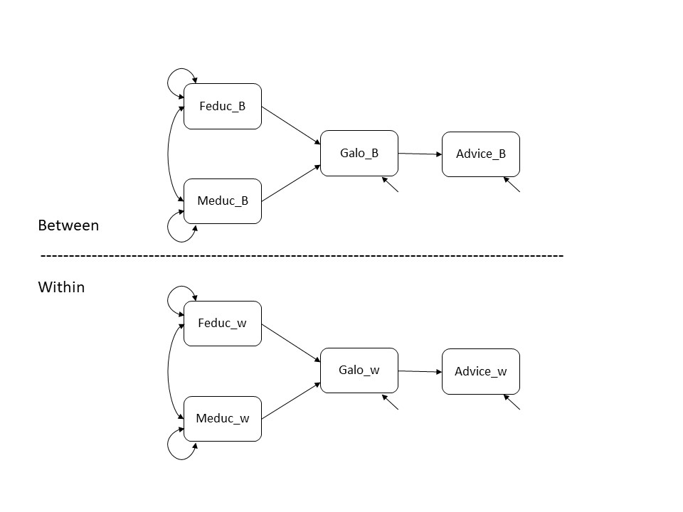
Figure 13.1: A two-level path diagram.
13.4 Obtaining ICCs, and estimates of \(\Sigma_\text{W}\) and \(\Sigma_\text{B}\)
In Script 13.1, we fit saturated models to Level 1 and Level 2, by letting all variables covary with each other at both levels. The means of the variables will be estimated only at Level 2 because Level-1 means are zero by definition. That is, Level-1 components of variables represent individual deviations from the cluster mean, and cluster-mean-centered variables have means of zero (both within clusters and across clusters). Fitting a saturated model will give us estimates of the within-level and between-level covariance matrices. The variance estimates from this model can be used to calculate ICCs. Fitting this model thus serves as a first step to obtain information about the variance distribution across levels.
Script 13.1
##   school galo advice feduc meduc
## 1      1   78      1     1     1
## 2      1  104      4     4     3
## 3      1   93      2     1     1
## 4      1  114      4     2     1
## 5      1   95      2     2     2
## 6      1   98      2     1     1
satmodel <- '
level: 1
galo ~~ advice + feduc + meduc
advice ~~ feduc + meduc
feduc ~~ meduc
level: 2
galo ~~ advice + feduc + meduc
advice ~~ feduc + meduc
feduc ~~ meduc
galo ~ 1
advice ~ 1
feduc ~ 1
meduc ~ 1
'
fitsat <- lavaan(model = satmodel, data = data, cluster = "school",
auto.var = TRUE)The clustering variable should be specified as an argument to the lavaan() function. The keywords level: 1 (not level 1:) and level:2 (not level 2:, which would return an error) identify blocks in the model syntax, notifying lavaan that we are specifying a model at each level of analysis. If the model syntax does not contain separate models for levels 1 and 2, but the clustering variable is still specified, then lavaan will fit a single-level model and report cluster-robust \(SE\)s and fit statistics.
One can obtain the ICC estimates for each variable, and the estimated covariance matrices at Level 1 and Level 2 from the saturated (or any) multilevel model using the following code.
##   galo advice  feduc  meduc
## 0.156 0.143 0.293 0.211## galo advice feduc meduc
## galo 143.572
## advice 12.802 1.730
## feduc 6.935 0.767 4.425
## meduc 5.901 0.704 2.265 3.764## galo advice feduc meduc
## galo 26.464
## advice 2.607 0.289
## feduc 5.737 0.669 1.833
## meduc 4.133 0.470 1.345 1.009The ICC values show that a proportion 0.156 of the total variance in the GALO achievement test scores as attributable to between-school differences. This could also be calculated manually using the variance estimates at the two levels (26.491 / (26.491 + 143.595) = .156). Educational level of the father has the largest proportion of between-school variance with an ICC of 0.293.
13.5 Fitting a two-level path model
In Script 13.2, we fit the two-level path model as depicted in Figure 13.1 to the data.
Script 13.2
model2 <- '
         level: 1
            advice ~ galo
            galo ~ feduc + meduc

            # covariance and variances
            feduc ~~ meduc

            advice ~~ advice
            galo ~~ galo
            feduc ~~ feduc
            meduc ~~ meduc

        level: 2
            advice ~ galo
            galo ~ feduc + meduc

            # covariance and variances
            feduc ~~ meduc

            advice ~~ advice
            galo ~~ galo
            feduc ~~ feduc
            meduc ~~ meduc

            galo ~ 1
            advice ~ 1
            feduc ~ 1
            meduc ~ 1
    '

fitmod2 <- lavaan(model = model2, data = data, cluster = "school")
Note that this two-level path model has \(df=4\). In two-level models, the number of observed statistics are twice as much as in single level models because we count the information at both levels. At the within level there are 4*(4+1)/2 = 10 elements in the within-level covariance matrix, and at the between level there are also 10 elements in the between-level covariance matrix (and there are four observed means). In this example, the number of parameters to be estimated is also doubled in comparison with a single level model, because all \(\beta\) and \(\psi\) parameters are estimated at the within as well as at the between-level. The number of parameters may also be different across levels, when a different model is fitted to the between level and to the within level. But in this model, we estimate three \(\beta\) parameters and five \(\psi\) parameters at each level, leading to \(df=2\) per level. At the between-level there are also four intercepts (\(\alpha\)) estimated based on four observed means, so the mean structure is saturated and does not add any \(df\) to the model.
## lavaan 0.6-20.2318 ended normally after 105 iterations
##
##   Estimator                                         ML
##   Optimization method                           NLMINB
##   Number of model parameters                        20
##
##   Number of observations                          1377
##   Number of clusters [school]                       58
##
## Model Test User Model:
##
##   Test statistic                                38.935
##   Degrees of freedom                                 4
##   P-value (Chi-square)                           0.000
##
## Model Test Baseline Model:
##
##   Test statistic                              2349.154
##   Degrees of freedom                                12
##   P-value                                        0.000
##
## User Model versus Baseline Model:
##
##   Comparative Fit Index (CFI)                    0.985
##   Tucker-Lewis Index (TLI)                       0.955
##
## Loglikelihood and Information Criteria:
##
##   Loglikelihood user model (H0)             -12612.714
##   Loglikelihood unrestricted model (H1)     -12593.247
##
##   Akaike (AIC)                               25265.428
##   Bayesian (BIC)                             25369.982
##   Sample-size adjusted Bayesian (SABIC)      25306.450
##
## Root Mean Square Error of Approximation:
##
##   RMSEA                                          0.080
##   90 Percent confidence interval - lower         0.058
##   90 Percent confidence interval - upper         0.103
##   P-value H_0: RMSEA <= 0.050                    0.013
##   P-value H_0: RMSEA >= 0.080                    0.522
##
## Standardized Root Mean Square Residual (corr metric):
##
##   SRMR (within covariance matrix)                0.028
##   SRMR (between covariance matrix)               0.046
##
## Parameter Estimates:
##
##   Standard errors                             Standard
##   Information                                 Observed
##   Observed information based on                Hessian
##
##
## Level 1 [within]:
##
## Regressions:
##                    Estimate  Std.Err  z-value  P(>|z|)
##   advice ~
##     galo              0.089    0.002   50.305    0.000
##   galo ~
##     feduc             1.092    0.180    6.060    0.000
##     meduc             0.918    0.195    4.706    0.000
##
## Covariances:
##                    Estimate  Std.Err  z-value  P(>|z|)
##   feduc ~~
##     meduc             2.261    0.128   17.622    0.000
##
## Variances:
##                    Estimate  Std.Err  z-value  P(>|z|)
##    .advice            0.589    0.023   25.680    0.000
##    .galo            131.155    5.125   25.589    0.000
##     feduc             4.425    0.172   25.687    0.000
##     meduc             3.768    0.146   25.744    0.000
##
##
## Level 2 [school]:
##
## Regressions:
##                    Estimate  Std.Err  z-value  P(>|z|)
##   advice ~
##     galo              0.104    0.007   14.958    0.000
##   galo ~
##     feduc            10.769   16.594    0.649    0.516
##     meduc           -10.290   22.314   -0.461    0.645
##
## Covariances:
##                    Estimate  Std.Err  z-value  P(>|z|)
##   feduc ~~
##     meduc             1.359    0.280    4.853    0.000
##
## Intercepts:
##                    Estimate  Std.Err  z-value  P(>|z|)
##    .galo             89.913    2.300   39.093    0.000
##    .advice           -7.489    0.711  -10.538    0.000
##     feduc             3.860    0.188   20.512    0.000
##     meduc             2.850    0.143   19.899    0.000
##
## Variances:
##                    Estimate  Std.Err  z-value  P(>|z|)
##    .advice            0.028    0.010    2.667    0.008
##    .galo              5.620    5.141    1.093    0.274
##     feduc             1.843    0.380    4.845    0.000
##     meduc             1.015    0.218    4.665    0.000
In the output, lavaan reports an overall test statistic, and several fit measures that are based on the overall model. The SRMR is provided separately for the within and between levels. For the current model exact fit is rejected, the RMSEA is 0.08 with a 90% confidence interval ranging from 0.058 to 0.103, and the CFI (for which the baseline model is the independence model at both levels) is 0.985.
The output for the parameter estimates is provided first for the within-level part of the model, and then for the between-level part. Interpretations depend on the level of analysis. For example:
- The effect of
galoonadviceis estimated to be .089 at the within-level. This means that whengaloscores increase by 1 point among individuals from the same school (i.e., \(\eta_{ij} = \mathrm{y}_{ij} - \mu_j\)), individuals are expected to receive 0.089 points higher advice on average. - The effect of
galoonadviceat the between-level is estimated to be .104. This means that when a school’s averagegaloscore (i.e., \(\mu_j\)) increases by 1 point, the school is expected to receive 0.104 points higher advice on average.
The difference between a variable’s between- and within-level effect (\(\beta_\text{B} - \beta_\text{W}\)) is called the contextual effect (see Marsh et al., 2012). In our example, this is the effect on received advice of being in a school with 1-unit higher average galo scores (\(\mu_j\)), given an individual’s own galo score (\(\mathrm{y}_{ij}\)).
\[\begin{equation} \begin{split} \text{advice} &= \beta_\text{W} (\mathrm{y}_{ij} - \mu_j) + \beta_\text{B} \mu_j \\ &= \beta_\text{W} \mathrm{y}_{ij} - \beta_\text{W} \mu_j + \beta_\text{B} \mu_j \\ &= \beta_\text{W} \mathrm{y}_{ij} + (\beta_\text{B} - \beta_\text{W}) \mu_j \end{split} \end{equation}\]
The equivalence of within- and between-level effects can be tested by comparing a model in which the effects are constrained to be equal to a model in which they are estimated freely. Alternatively, one could define the contextual effect as a new parameter by subtracting the two effects of interest, similar to how one defines specific indirect effects.
' level: 1
    advice ~ b43.w*galo
  level: 2
    advice ~ b43.b*galo
b43.contextual := b43.b - b43.w   # obtain Wald z test of equivalence v. contextual effect'
In standard multilevel regression, one may also include random slopes in the model. This way one could test whether the effect of some variable on another variable varies across clusters. Random slopes are not yet a feature in lavaan’s multilevel SEM, although the wide-format approach might be feasible in samples with many small clusters (Barendse & Rosseel, 2020).
References
Barendse, M. T., & Rosseel, Y. (2020). Multilevel modeling in the ‘wide format’ approach with discrete data: A solution for small cluster sizes. Structural Equation Modeling, 27(5), 696–721. https://doi.org/10.1080/10705511.2019.1689366
Hox, J. J., Moerbeek, M., & Van de Schoot, R. (2017). Multilevel analysis: Techniques and applications. Routledge.
Marsh, H. W., Ludtke, O., Nagengast, B., Trautwein, U., Morin, A. J. S., Abduljabbar, A. S., et al. (2012). Classroom climate and contextual effects: Conceptual and methodological issues in the evaluation of group-level effects. Educational Psychololgy, 47, 106–124. https://doi.org/10.1080/00461520.2012.670488
Muthén, B. (1990). Mean and covariance structure analysis of hierarchical data. Los Angeles, CA: UCLA.
Muthén, B.O. (1994). Multilevel covariance structure analysis. Sociological Methods & Research, 22(3), 376–398. https://doi.org/10.1177%2F0049124194022003006
Williams, R. L. (2000). A note on robust variance estimation for cluster‐correlated data. Biometrics, 56(2), 645–646. https://doi.org/10.1111/j.0006-341X.2000.00645.x
Schijf, H., & Dronkers, J. (1991). De invloed van richting en wijk op de loopbanen in de lagere scholen van de stad Groningen in 1971. IBH Abram, BPM Creemers & A. van derLeij (red.), ORD, 91.
Schmidt, W. H. (1969). Covariance structure analysis of the multivariate random effects model [Doctoral dissertation]. University of Chicago, Department of Education.