21 Mean structures
Until now we have only addressed the analysis of covariance structure. However, we can also analyze mean structure using structural equation modeling. In the case of longitudinal or multigroup models, the analyses of means becomes especially relevant if the goal of the analysis is to compare means across groups or occasions.
We have shown the models for the covariances in both factor analysis and path analysis previously (see Chapters 3 and 14), but we have not yet shown the mean structure in those models. In this chapter we will first extent the models for factor analysis and path analysis to include the mean structure, and then explain how to model the mean structure in a factor model and in a path model in lavaan.
21.1 Mean structure of a factor model
Let’s reconsider the factor model that we used as an example in Chapter 14. The figure below is a graphical representation of the equations (21.1) through (21.9).
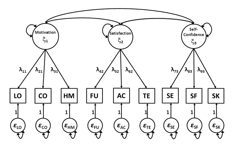
Figure 21.1: Factor model of the School Attitudes Questionnaire
\[\begin{align} \mathrm{x}_1 = \lambda_{11}\xi_1+\varepsilon_1, \tag{21.1} \\ \mathrm{x}_2 = \lambda_{21}\xi_1+\varepsilon_2, \tag{21.2} \\ \mathrm{x}_3 = \lambda_{31}\xi_1+\varepsilon_3, \tag{21.3} \\ \mathrm{x}_4 = \lambda_{42}\xi_2+\varepsilon_4, \tag{21.4} \\ \mathrm{x}_5 = \lambda_{52}\xi_2+\varepsilon_5, \tag{21.5} \\ \mathrm{x}_6 = \lambda_{62}\xi_2+\varepsilon_6, \tag{21.6} \\ \mathrm{x}_7 = \lambda_{73}\xi_3+\varepsilon_7, \tag{21.7} \\ \mathrm{x}_8 = \lambda_{83}\xi_3+\varepsilon_8, \tag{21.8} \\ \mathrm{x}_9 = \lambda_{93}\xi_3+\varepsilon_9, \tag{21.9} \end{align}\]
If we add the mean structure to the factor model, we arrive at the following equations:
\[\begin{align} \mathrm{x}_1 = \tau_{1} + \lambda_{11}\xi_1+\varepsilon_1, \tag{21.10} \\ \mathrm{x}_2 = \tau_{2} + \lambda_{21}\xi_1+\varepsilon_2, \tag{21.11} \\ \mathrm{x}_3 = \tau_{3} + \lambda_{31}\xi_1+\varepsilon_3, \tag{21.12} \\ \mathrm{x}_4 = \tau_{4} + \lambda_{42}\xi_2+\varepsilon_4, \tag{21.13} \\ \mathrm{x}_5 = \tau_{5} + \lambda_{52}\xi_2+\varepsilon_5, \tag{21.14} \\ \mathrm{x}_6 = \tau_{6} + \lambda_{62}\xi_2+\varepsilon_6, \tag{21.15} \\ \mathrm{x}_7 = \tau_{7} + \lambda_{73}\xi_3+\varepsilon_7, \tag{21.16} \\ \mathrm{x}_8 = \tau_{8} + \lambda_{83}\xi_3+\varepsilon_8, \tag{21.17} \\ \mathrm{x}_9 = \tau_{9} + \lambda_{93}\xi_3+\varepsilon_9, \tag{21.18} \end{align}\]
Equations (21.10) through (21.18) can also be written in matrix form:
\[\begin{equation} \mathbf{x} = \mathbf\tau + \Lambda \mathbf\xi+\varepsilon, \tag{21.19} \end{equation}\]where \(\mathbf{x}\) is a vector of all observed variables, \(\mathbf\xi\) is a vector of all common factors, \(\mathbf\varepsilon\) is a vector of all residual factors, \(\mathbf\Lambda\) is a matrix of factor loadings, and \(\mathbf\tau\) is a vector of intercepts: \[ \mathbf{x}= \begin{bmatrix} x_1\\x_2\\x_3\\x_4\\x_5\\x_6\\x_7\\x_8\\x_9 \end{bmatrix}, \mathbf\xi = \begin{bmatrix} \xi_1\\\xi_2\\\xi_3 \end{bmatrix}, \mathbf\varepsilon = \begin{bmatrix} \varepsilon_1\\\varepsilon_2\\\varepsilon_3\\\varepsilon_4\\\varepsilon_5\\\varepsilon_6\\\varepsilon_7\\\varepsilon_8\\\varepsilon_9 \end{bmatrix}, \mathbf\Lambda = \begin{bmatrix} \lambda_{11}&0&0\\\lambda_{21}&0&0\\\lambda_{31}&0&0\\0&\lambda_{42}&0\\0&\lambda_{52}&0\\0&\lambda_{62}&0\\0&0&\lambda_{73}\\0&0&\lambda_{83}\\0&0&\lambda_{93} \end{bmatrix}, \text{ and } \mathbf\tau = \begin{bmatrix} \tau_1\\\tau_2\\\tau_3\\\tau_4\\\tau_5\\\tau_6\\\tau_7\\\tau_8\\\tau_9 \end{bmatrix}. \]
The means of the common factors are represented by \(\text{MEAN}(\xi) = \mathbf\kappa\), the means of the residual factors are assumed zero, \(\text{MEAN}(\varepsilon) = 0\). With these assumptions we can derive expressions for the means of observed variables \(\mathbf{x}\), called \(\text{MEAN}(\mathbf{x}) = \mathbf{\mu}\),
\[\begin{equation} \mathbf\mu = \mathbf\tau + \mathbf\Lambda \mathbf\kappa \tag{21.20} \end{equation}\]where \(\mathbfμ\) (‘mu’) is a column vector of means of the observed variables, \(\mathbfτ\) (‘tau’) is a column vector of intercepts, \(\mathbfΛ\) is a matrix of factor loadings, and \(\mathbfκ\) (‘kappa’) is a column vector of means for the common factors. Derivations of Equation (21.20) are given in the Appendix at the end of this Chapter. Substitution of the \(\mathbf\tau\), \(\mathbf\Lambda\), and \(\mathbf\kappa\) of our example from Figure 21.1 yields:
\[\begin{equation} \mathbf\mu = \begin{bmatrix} \mu_1\\\mu_2\\\mu_3\\\mu_4\\\mu_5\\\mu_6\\\mu_7\\\mu_8\\\mu_9 \end{bmatrix} = \begin{bmatrix} \tau_1 + \lambda_{11}\kappa_1\\ \tau_2 + \lambda_{21}\kappa_2\\ \tau_3 + \lambda_{31}\kappa_3\\ \tau_4 + \lambda_{41}\kappa_4\\ \tau_5 + \lambda_{51}\kappa_5\\ \tau_6 + \lambda_{61}\kappa_6\\ \tau_7 + \lambda_{71}\kappa_7\\ \tau_8 + \lambda_{81}\kappa_8\\ \tau_9 + \lambda_{91}\kappa_9 \end{bmatrix}, \tag{21.21} \end{equation}\]or \(\mathbf\mu_{\text{population}} = \mathbf\mu_{\text{model}}\).
21.2 Mean structure of a path model
If we go back to the path model from Chapter 3 (see Figure 21.2), and include the mean structure, we arrive at the following equations:
\[\begin{align} \mathrm{y}_1 & = \alpha_1 + \zeta_1, \tag{21.22} \\ \mathrm{y}_2 & = \alpha_2 + \zeta_2 , \tag{21.23} \\ \mathrm{y}_3 & = \alpha_3 + \beta_{31}\mathrm{y}_1 + \beta_{32}\mathrm{y}_2 + \zeta_3 \tag{21.24} \\ \mathrm{y}_4 & = \alpha_4 + \beta_{43}\mathrm{y}_3 + \zeta_44 , \tag{21.25} \\ \end{align}\]
where \(\mathrm{y}_1\), \(\mathrm{y}_2\), \(\mathrm{y}_3\), and \(\mathrm{y}_4\) are observed variables, \(\zeta_1\), \(\zeta_2\), \(\zeta_3\) and \(\zeta_4\) are residual factors, \(\alpha_1\) \(\alpha_2\), \(\alpha_3\), and \(\alpha_4\) are intercepts, and \(\beta_{31}\), \(\beta_{32}\), and \(\beta_{43}\) are regression coefficients.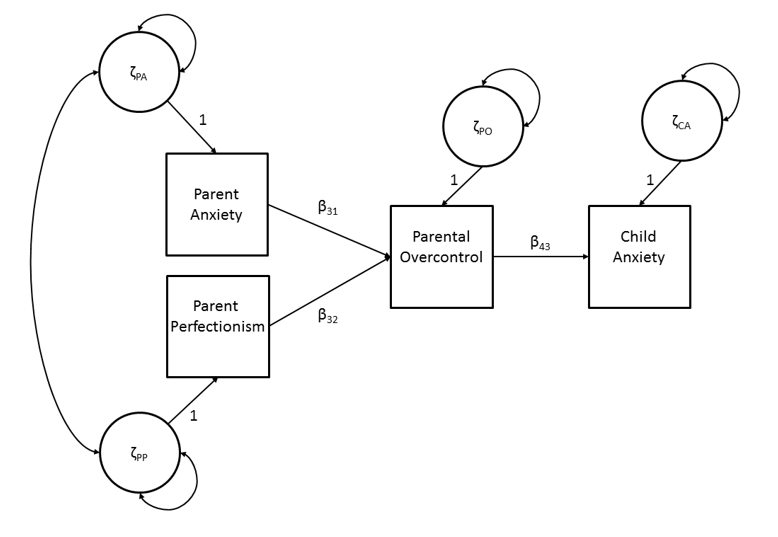
Figure 21.2: Path model of child anxiety.
Equations (21.22) through (21.25) can also be written in matrix form:
\[\begin{equation} \mathbf{y} = \mathbf\alpha+\mathbf{B}\mathbf{y}+\mathbf\zeta \tag{21.26} \end{equation}\]where \(\mathbf{y}\) is a vector of all observed variables, \(\mathbf\zeta\) is a vector of all residual factors, \(\mathbf\alpha\) is a vector of intercepts, and \(\mathbf{B}\) is a matrix of regression coefficients,
\[ \mathbf{y} = \begin{bmatrix}\mathrm{y}_1\\ \mathrm{y}_2\\ \mathrm{y}_3 \\ \mathrm{y}_4 \end{bmatrix}, \mathbf\zeta = \begin{bmatrix} \zeta_1 \\ \zeta_2 \\ \zeta_3 \\ \zeta_4 \end{bmatrix}, \mathbf\alpha = \begin{bmatrix} \alpha_1 \\ \alpha_2 \\ \alpha_3 \\ \alpha_4 \end{bmatrix}, \text{ and }\mathbf{B} = \begin{bmatrix} 0 & 0 & 0 & 0 \\ 0 & 0 & 0 & 0 \\ \beta_{31} & \beta_{32} & 0 & 0 \\ 0 & 0 & \beta_{43} & 0 \end{bmatrix}. \]
We assume the residual factors have zero means: \(\text{MEAN}(\mathbf\zeta) = 0\).
In order to find the model for the means of the observed variables, we first have to rewrite \(\mathbf{y}\) in Equation (21.26) as a function of model parameters.
\[\begin{align} \mathbf{y} &= \mathbf\alpha + \mathbf{B} \mathbf{y} + \mathbf\zeta \Leftrightarrow \\ \mathbf{y} &= (\mathbf{I} - \mathbf{B})^{-1} \mathbf\alpha + (\mathbf{I} - \mathbf{B})^{-1} \mathbf\zeta, \tag{21.27} \end{align}\]
Now, using covariance algebra we can find expressions for the means of \(\mathrm{y}\)y, called \(\mathbf{\mu} = \text{MEAN}(\mathrm{y})\),
\[\begin{equation} \mathbf{\mu} = (\mathbf{\text{I}} - \mathbf{\text{B}})^{-1}\hspace{1mm}\mathbf\alpha. \tag{21.28} \end{equation}\]Derivations of Equations (21.27) and (21.28) are given in Appendix 1, at the end of this Chapter. Substituting the \(\mathbf\alpha\) and \(\mathbf{\text{B}}\) of our example from Figure 21.2 we obtain:
\[\begin{equation} \mathbf{\mu} = \begin{bmatrix} \mu_1 \\ \mu_2 \\ \mu_3 \\ \mu_4 \end{bmatrix} = \begin{bmatrix} \alpha_1\\ \alpha_2\\ \alpha_3 + \beta_{31} \alpha_1 + \beta_{32}\alpha_2\\ \alpha_4 + \beta_{43}(\alpha_3 + \beta_{31}\alpha_1 + \beta_{32}\alpha_2) \end{bmatrix}, \tag{21.29} \end{equation}\]or \(\mathbf\mu_{\text{population}} = \mathbf{\mu}_{\text{model}}\)
21.3 Mean structure of a factor model in lavaan
The model for the means in a factor model is \(\mathbf\mu = \mathbf\tau + \mathbf\Lambda \mathbf\kappa.\) In this equation, \(\mathbfμ\) (‘mu’) is a column vector of means of the observed variables, \(\mathbfτ\) (‘tau’) is a column vector of intercepts, \(\mathbfΛ\) is the usual full matrix of factor loadings, and \(\mathbfκ\) (‘kappa’) is a column vector of means for the common factors. For our example of the SAQ measurement model from Chapter 14, the model looks like this:
\[ \mathbf\mu = \begin{bmatrix} \mu_1\\\mu_2\\\mu_3\\\mu_4\\\mu_5\\\mu_6\\\mu_7\\\mu_8\\\mu_9\\ \end{bmatrix}=\begin{bmatrix} \tau_1\\\tau_2\\\tau_3\\\tau_4\\\tau_5\\\tau_6\\\tau_7\\\tau_8\\\tau_9\\ \end{bmatrix}+\begin{bmatrix} \lambda_{11}&0&0\\ \lambda_{21}&0&0\\ \lambda_{31}&0&0\\ 0&\lambda_{42}&0\\ 0&\lambda_{52}&0\\ 0&\lambda_{62}&0\\ 0&0&\lambda_{73}\\ 0&0&\lambda_{83}\\ 0&0&\lambda_{93}\\ \end{bmatrix}\begin{bmatrix} \kappa_1\\\kappa_2\\\kappa_3\\ \end{bmatrix} \]
In the model for the covariances, we had to give scale to the common factor, either by fixing the factor variances at a nonzero value (typically 1) or by constraining factor loadings (e.g., fix one loading per factor to 1, or constrain a factor’s loadings to have a mean of 1). In the model for the means, we need to give the common factors an ‘origin’23. We do this in a way that is analogous to identifying the scale of a factor:
We can fix the factor mean to 0, which is analogous to fixing the factor variance to 1. This “fixed-factor” method reflects a choice to interpret common factors as having a standard normal distribution, like z scores.
We can fix one intercept per factor to 0. This gives the latent mean the same mean as that reference variable, and other indicator intercepts are interpreted relative to that mean.
We can constrain a factor’s intercepts to have an average (or sum) of zero. This has the effect of giving the factor a mean that is the grand mean across indicators. All indicator intercepts are interpreted relative to that grand mean.
Script 21.1 is analogous to Script 14.1, but it fits the measurement model of the SAQ with a mean structure. Scale and origin are given through common factor variances and means (by fixing elements in \(\mathbfΦ\) and \(\mathbfκ\)).
Script 21.1
## observed data
## observed covariance matrix
obsnames <- c("learning","concentration","homework","fun",
            "acceptance","teacher","selfexpr","selfeff","socialskill")
values <- c(30.6301,
            26.9452, 56.8918,
            24.1473, 31.6878, 53.2488,
            16.3770, 18.4153, 16.8599, 27.9758,
             7.8174,  9.6851, 12.0114, 12.8765, 47.0970,
            13.6902, 16.9232, 12.9326, 17.2880, 12.3672, 29.0119,
            15.3122, 24.2849, 21.4935, 12.9621, 13.9909, 11.6333, 59.5343,
            13.4457, 21.8158, 18.8545,  7.3931, 12.2333,  7.1434, 29.7953, 49.2213,
             6.6074, 12.7343, 12.5768,  6.4065, 13.4258,  6.1429, 26.0849, 23.6253, 40.0922)

saqcov <- getCov(values, names = obsnames)
## means
saqmeans <- c(39.7346, 36.1846, 37.4528, 42.9006, 41.3240, 41.4077,
              35.7519, 35.6172, 38.9092)
names(saqmeans) <- obsnames

## define model including mean structure
## scale and locate by fixing common factor variances and means
saqmodel <- '## MODEL COVARIANCE STRUCTURE
    # define latent common factors
    Motivation =~ L11*learning + L21*concentration + L31*homework
    Satisfaction =~ L42*fun + L52*acceptance + L62*teacher
    SelfConfidence =~ L73*selfexpr + L83*selfeff + L93*socialskill

    # indicator residual variances (or use "auto.var = TRUE")
    learning ~~ TH11*learning
    concentration ~~ TH22*concentration
    homework ~~ TH33*homework
    fun ~~ TH44*fun
    acceptance ~~ TH55*acceptance
    teacher ~~ TH66*teacher
    selfexpr ~~ TH77*selfexpr
    selfeff ~~ TH88*selfeff
    socialskill ~~ TH99*socialskill

    # common factor variances (or use "auto.var = TRUE")
      Motivation ~~ F11*Motivation
      Satisfaction ~~ F22*Satisfaction
      SelfConfidence ~~ F33*SelfConfidence
    # factor covariances (or use "auto.cov.lv.x = TRUE")
    Motivation ~~ F21*Satisfaction
    Motivation ~~ F31*SelfConfidence
    Satisfaction ~~ F32*SelfConfidence

    # OPTIONAL: fix factor variances (or use "std.lv = TRUE")
    F11 == 1
    F22 == 1
    F33 == 1

## MODEL MEAN STRUCTURE
    # intercepts observed variables
    learning ~ T1*1
    concentration ~ T2*1
    homework ~ T3*1
    fun ~ T4*1
    acceptance ~ T5*1
    teacher ~ T6*1
    selfexpr ~ T7*1
    selfeff ~ T8*1
    socialskill ~ T9*1

    # means common factors
    Motivation ~ K1*1
    Satisfaction ~ K2*1
    SelfConfidence ~ K3*1

    # OPTIONAL: manually specify location constraints
    # fixed-factor method (default in lavaan, not needed in syntax)
        K1 == 0
        K2 == 0
        K3 == 0
    # marker- / reference-variable method (MUST specify in syntax)
        # T1 == 0
        # T4 == 0
        # T7 == 0
    # effects-coding method (MUST specify in syntax)
      # NOTE: 3 different ways yield the same solution
    # (T1 + T2 + T3) / 3 == 0 # mean(τ) = 0
    # T4 + T5 + T6 == 0       # sum(τ) = 0
    # T7 == 0 – T8 – T9       # 1 τ = negative sum of remaining τ
'

## fit model
saqmodelOut <- lavaan(saqmodel, sample.cov = saqcov,
                      sample.mean = saqmeans, sample.nobs = 915,
                      likelihood = "normal", fixed.x = FALSE)
## results
summary(saqmodelOut)
## parameter matrices
lavInspect(saqmodelOut, "est")
We first define our observed data. In this case, we have to define the means of our observed data in addition to the covariance. The object saqmeans now contains the means of the nine observed variables, and we provide variable labels using the function names().
saqmeans <- c(39.7346, 36.1846, 37.4528, 42.9006, 41.3240, 41.4077,
              35.7519, 35.6172, 38.9092)
names(saqmeans) <- obsnames
In the model specification we have to define the parameters for the model of the means, in addition to the parameters that are defined for the model of the variances and covariances. We have split the specification of the saqmodel into a section “MODEL COVARIANCE STRUCTURE” and “MODEL MEAN STRUCTURE” to emphasize this distinction. The model for the covariances is equal to the model that we used for the measurement model of the SAQ in Chapter 12. We give scales to the common factors by fixing the common factor variances at 1.
The model for the means includes the intercept parameters of the observed indicators (\(τ\)) and the common factor means (\(κ\)). To define these parameters we use the tilde sign (~) in combination with a ‘1’. This combination (~ 1) specifies that we want to define the mean structure of our model, where the mean structure is represented as regressing a variable onto a constant ‘1’. Recall that this is also how to specify an intercept-only model using ordinary least-squares regression: lm(learning ~ 1).
    ## MODEL MEAN STRUCTURE
    # intercepts observed variables
    learning ~ T1*1
    concentration ~ T2*1
    homework ~ T3*1
    fun ~ T4*1
    acceptance ~ T5*1
    teacher ~ T6*1
    selfexpr ~ T7*1
    selfeff ~ T8*1
    socialskill ~ T9*1

    # means common factors (exclude if relying on lavaan's default)
    Motivation ~ K1*1
    Satisfaction ~ K2*1
    SelfConfidence ~ K3*1
The labels that we use here refer to the position of the parameter estimate in the vector of intercepts (“T1” to “T9” in tau) and the vector of common factor means (“K1” to “K3’ in kappa). We then use these labels to impose the necessary identification constraints. Here, we freely estimate all intercepts, but we constrain all common factor means to zero. Note that lavaan constrains common-factor means by default, so the factor means and their constraints could be omitted from the model syntax.
    # fixed-factor method (default in lavaan, not needed in syntax)
    K1 == 0
    K2 == 0
    K3 == 0
When we run the model using the lavaan() function, we have to provide the observed means in addition to the other elements.
saqmodelOut <- lavaan(saqmodel, sample.cov = saqcov,
                      sample.mean = saqmeans, sample.nobs = 915,
                      likelihood = "normal", fixed.x = FALSE)
Note that we are now using “normal” likelihood instead of “Wishart” likelihood because we are including the mean structure. This still means that we rely on the assumption that our observed data are normally distributed in the population, but the underlying statistical theory is based on the sampling variability of actual data vectors (\(\mathrm{y}\)) instead of the sampling variability of covariance matrices (\(\mathbf\Sigma\)). One practical consequence of this distinction is that we calculate our standard errors and \(χ^2\) test statistic using \(N\) instead of \(N – 1\) in our formulas. Results will be indistinguishable in asymptotically large samples, but you will notice minor differences in smaller samples. The point is simply that a Wishart distribution only describes the sampling variability of covariance matrices, not of mean vectors, so it is not appropriate to use Wishart likelihood when modeling mean and covariance structure (although it is valid to use normal likelihood even if you only model the covariance structure). Note that lavaan uses normal likelihood by default, so when fitting a model to a mean vector or to raw data, you can leave out the likelihood argument.
The output will now give us an additional part named “Intercepts” that displays both the parameter estimates of the intercepts of the observed indicators and of the common factors. Note that intercepts of exogenous variables are means because the model of an exogenous variable is an intercept-only model. Like residual variances, the intercepts of endogenous variables are denoted with a “.” prefix.
                   Estimate  Std.err  Z-value  P(>|z|)
Intercepts:
   .learning  (T1)   39.735    0.183  217.292    0.000
   .concntrtn (T2)   36.185    0.249  145.193    0.000
   .homework  (T3)   37.453    0.241  155.338    0.000
   .fun       (T4)   42.901    0.175  245.482    0.000
   .acceptanc (T5)   41.324    0.227  182.244    0.000
   .teacher   (T6)   41.408    0.178  232.670    0.000
   .selfexpr  (T7)   35.752    0.255  140.237    0.000
   .selfeff   (T8)   35.617    0.232  153.650    0.000
   .socilskll (T9)   38.909    0.209  185.982    0.000
    Motivatin (K1)    0.000
    Satisfctn (K2)    0.000
    SlfCnfdnc (K3)    0.000
In this case, the mean structure of our model is just-identified. Thus, the parameter estimates of the intercepts of the observed indicators equal the observed means. Thus, the model fit, χ2(24) = 184.04, p < .001, is identical to the results from Script 12.1, which modeled covariance structure only.
Script 21.1 also shows how to provide an origin for the common factors via intercepts (by fixing or constraining elements in τ). There is no lavaan argument to do these by default, so these options must be specified in the model syntax.
    # marker- / reference-variable method (MUST specify in syntax)
        # T1 == 0
        # T4 == 0
        # T7 == 0
    # effects-coding method (MUST specify in syntax)
      # NOTE: 3 different ways yield the same solution
    # (T1 + T2 + T3) / 3 == 0 # mean(τ) = 0
    # T4 + T5 + T6 == 0       # sum(τ) = 0
    # T7 == 0 – T8 – T9       # 1 τ = negative sum of remaining τ
Note that identification of mean structure is independent of identification of covariance structure (unless data are categorical; see Chapter 25). So you can use the fixed-factor method to identify factor means even if you use a reference variable or effects coding to identify factor variances.
21.4 Mean structure of a path model
The model for the means in a path model are given by \(\mathbf\mu = (\mathbf{\text{I}} − \textbf{B})^{−1} \mathbf\alpha,\) where \(\mathbfμ\) (‘mu’) is a column vector of means of the observed variables, matrix \(\textbf{B}\) is the usual full matrix of direct effects between the observed variables, and \(\mathbf\alpha\) (‘alpha’) is a column vector of intercepts. For our example of the child anxiety model from Chapter 3, the model looks like this:
\[ \mathbf\mu = \begin{bmatrix} \mu_1\\\mu_2\\\mu_3\\\mu_4\\ \end{bmatrix} = \begin{pmatrix} \begin{bmatrix} 1&0&0&0\\0&1&0&0\\0&0&1&0\\0&0&0&0\\ \end{bmatrix} - \begin{bmatrix} 0&0&0&0\\0&0&0&0\\\beta_{31}&\beta_{32}&0&0\\0&0&\beta_{43}&0\\ \end{bmatrix} \end{pmatrix} ^{-1} \begin{bmatrix} \alpha_1\\\alpha_2 \\ \alpha_3 \\ \alpha_4\\ \end{bmatrix} , \]
If we would like to add the mean structure to our path model from Chapter 3, we have to define the intercepts in our model (using the ‘~1’ operator, just as we did in the factor model), and we would have to provide the vector of observed means in the lavaan() function (using sample.mean = AWmeans). Again, in this situation the model for the means is just-identified.
The mean structure of a path model can also be applied in structural regression models. When the means are modeled in a structural regression model, not only the covariances but also the means of the common factors are modeled using a path model. In this case, both the covariance matrix of the common factors (\(\mathbfΦ\)) and the means of the common factors (\(\mathbfκ\)) are estimated as a function of parameters from a path model, using \(\mathbfΦ = (\textbf{I} − \textbf{Β})^{−1} \mathbfΨ (\textbf{I} − \textbf{Β})^{−1\text{T}}\) and \(\mathbfκ = (\textbf{I} − \textbf{Β})^{−1} \mathbf\alpha\). Thus, just as the covariance structure of a full SEM is \(\mathbf\Sigma_{\text{model}} = \mathbf\Lambda (\textbf{I} − \textbf{Β})^{−1} \mathbf{Ψ} (\textbf{I} − \textbf{Β})^{−1\text{T}} \mathbf\Lambda^{\text{T}} + \mathbf\Theta\), the mean structure of a full SEM is \(\mathbf\Sigma_{\text{model}} = \mathbf\tau + \mathbf\Lambda (\textbf{I} − \textbf{B})^{−1} \mathbf\alpha\).
Appendix
Derivations of equation (21.20), (21.27), and (21.28).
Derivation of Equation 21.20
\[\begin{align} \mathbf\mu &= \text{MEAN}(\mathrm{x}) \Leftrightarrow \\ & (\text{substitute Equation 21.19}) \\ \mathbf\mu &= \text{MEAN}(\mathbf\tau + \mathbf\Lambda \mathbf\xi + \mathbf\varepsilon) \Leftrightarrow\\ & (\text{mean of sum equals the sum of means}) \\ \mathbf\mu &= \text{MEAN}(\mathbf\tau) + \text{MEAN}(\mathbf\Lambda \mathbf\xi) + \text{MEAN}(\mathbf\varepsilon)) \Leftrightarrow \\ & (\text{mean of a constant equals the constant}) \\ \mathbf\mu &= \mathbf\tau + \mathbf\Lambda \text{MEAN}(\mathbf\xi) + \text{MEAN}(\mathbf\varepsilon) \Leftrightarrow \\ & (\text{means of } \mathbf\xi \text{ are given by } \mathbf\kappa \text{, and means of } \mathbf\varepsilon \text{ are assumed zero)} \\ \mathbf\mu &= \mathbf\tau + \mathbf\Lambda \mathbf\kappa \\ \end{align}\]
Derivation of Equation 21.27
\[\begin{align} \mathrm{y} &= \mathbf\alpha + \textbf{B}\mathrm{y} + \mathbf\zeta \Leftrightarrow \\ \mathrm{y} − \textbf{B}\mathrm{y} &= \mathbf\alpha + \mathbf\zeta \Leftrightarrow \\ \textbf{I}\mathrm{y} − \textbf{B}\mathrm{y} &= \mathbf\alpha + \mathbf\zeta \Leftrightarrow \\ (\textbf{I} − \textbf{B})\mathrm{y} &= \mathbf\alpha + \mathbf\zeta \Leftrightarrow \\ \end{align}\]
(premultiply both sides by \((\textbf{I} − \textbf{B})^{−1}\))
\[\begin{align} (\textbf{I} − \textbf{B})^{−1} (\textbf{I} − \textbf{B})\mathrm{y} &= (\textbf{I} − \textbf{B})^{−1} (\mathbf\alpha + \mathbf\zeta )\Leftrightarrow \\ \mathrm{y} &= (\textbf{I} − \textbf{B})^{−1} (\mathbf\alpha + \mathbf\zeta) \Leftrightarrow \\ \mathrm{y} &= (\textbf{I} − \textbf{B})^{−1} \mathbf\alpha + (\textbf{I} − \textbf{B})^{−1} \mathbf\zeta \\ \end{align}\]
Derivation of Equation 21.28
\[\begin{align} \mathbf\mu &= \text{MEAN}(\mathrm{y}) \Leftrightarrow \\ &(\text{substitute Equation 21.27})\\ \mathbf\mu &= \text{MEAN}((\textbf{I} − \textbf{B})^{−1} \mathbf\alpha + (\textbf{I} − \textbf{B})^{−1} \mathbf\zeta) \Leftrightarrow \\ &(\text{mean of sum equals the sum of means})\\ \mathbf\mu &= \text{MEAN}((\textbf{I} − \textbf{B})^{−1} \mathbf\alpha) + \text{MEAN}((\textbf{I} − \textbf{B})^{−1} \mathbf\zeta) \Leftrightarrow \\ &(\text{mean of a constant equals the constant)}\\ \mathbf\mu &=(\textbf{I} − \textbf{B})^{−1} \mathbf\alpha + (\textbf{I} − \textbf{B})^{−1} \text{MEAN} (\mathbf\zeta) \Leftrightarrow \\ &(\text{means of } \mathbf\zeta \text{ are assumed zero})\\ \mathbf\mu &= (\textbf{I} − \textbf{B})^{−1} \mathbf\alpha + (\textbf{I} − \textbf{B})^{−1} 0 \Leftrightarrow\\ \mathbf\mu &=(\textbf{I} − \textbf{B})^{−1} \mathbf\alpha \\ \end{align}\]
Think of this as a ‘location’ on the number line where we put the center of our latent variable’s distribution, and we scale it by deciding how spread out around that location the distribution is.↩︎