7 Identification
The problem of identification considers the issue of whether there is enough “known” information to obtain unique estimates of the model that is specified (i.e., the “unknown” information). In structural equation modeling, the known pieces of information are the sample variances and covariances of the observed variables, and the unknown pieces of information are the model parameters. When the model is “underidentified”, this means that there is not enough known information to yield unique parameter estimates. When there are just as many knowns as unknowns, the model is “just identified”. However, usually we are interested in so called “overidentified” models, where there are more knowns than unknowns. Identification is an important but rather difficult topic of structural equation modeling, and there are many different ways to evaluate the identification status of a model.
The first, and easiest way to evaluate whether a model might be identified is to evaluate whether the number of model parameters to be estimated is equal to or smaller than the number of nonredundant elements in the observed covariance matrix:
\[\begin{equation} q \le (p(p+1)) ½, \tag{7.1} \end{equation}\]where \(p\) is the number of observed variables, and \(q\) is the number of free parameters in the model. This is a general rule that can be applied to all structural equation models. However, it is a ‘necessary but not sufficient’ condition for identification. This means that models that have a negative number of degrees of freedom are surely not identified. Models that have at least zero degrees of freedom might be identified. Evaluation of Equation (7.1) for our illustrative example of child anxiety yields a total of 10 knowns (i.e., \(p = 4\)), and 8 unknowns (i.e., \(\beta_{31}\), \(\beta_{32}\), \(\beta_{43}\), \(\psi_{11}\), \(\psi_{22}\), \(\psi_{33}\), \(\psi_{44}\) and \(\psi_{21}\)). The difference between the number or nonredundant elements in the covariance matrix and the number of free parameters in the model are the ‘degrees of freedom’. The model of our example thus has 2 degrees of freedom.
There are different approaches to further assess whether a model is identified. In this chapter we will first discuss the symbolic or theoretical identification of model parameters. In addition, we will explain some rules of thumb that can be applied in order to facilitate the evaluation of model identification. We only discuss identification of path models, identification of factor models will be discussed in a later chapter.
Some conditions related to identification are sufficient, which means that if the condition holds, the model is surely identified (at least theoretically), but there may be other identified models for which the condition does not hold. Other conditions are necessary, which means that if the condition holds, the model might be identified. If a necessary condition doesn’t hold, the model is surely not identified.
7.1 Assessment of identification using the elements of \(\mathbf\Sigma_{\text{population}}\) and \(\mathbf\Sigma_{\text{model}}\)
A model is identified only when all unknown parameters of the model are identified. Identification of model parameters can be demonstrated by showing that the unknown parameters are functions of known parameters, i.e., that we can give a description of the free parameters in the model in terms of population variances and covariances (\(\mathbf\Sigma_{\text{population}}\)). The population variances and covariances are known-to-be-identified (i.e., known information) because the observed sample variances and covariances (\(\mathbf\Sigma_{\text{sample}}\)) are direct estimates of \(\mathbf\Sigma_{\text{population}}\). Therefore, if an unknown parameter can be written as a function of one or more elements of \(\mathbf\Sigma_{\text{population}}\), then that parameter is identified.
As an example, we take \(\mathbf\Sigma_{\text{model}}\) from Equation (3.10). Here, the elements of the covariance matrix are written as a function of model parameters. In order to evaluate the identification status of a parameter, we need to write the equation the other way around, so that the model parameter is a function of population variances and covariances. If each unknown model parameter can be written as a function of known parameters, then the model of Equation (3.10) is identified. For example, the first three elements of the model implied covariance matrix are a function of single model parameters \(ψ_{11}\), \(ψ_{22}\), and \(ψ_{21}\). These parameters can therefore be represented by the population variances \(\sigma_{11}\), \(\sigma_{22}\), and covariance \(\sigma_{21}\):
\[\begin{equation} \psi_{11} = \sigma_{11} \tag{7.2} \end{equation}\]
\[\begin{equation} \psi_{22} = \sigma_{22} \tag{7.3} \end{equation}\]
\[\begin{equation} \psi_{21} = \sigma_{21} \tag{7.4} \end{equation}\]
These equations thus have the same number of “knowns” as “unknowns’, which leads to a unique expression for each model parameter. The parameters \(ψ_{11}\), \(ψ_{22}\), and \(ψ_{21}\) are thus identified.
The equations for the population covariances \(\sigma_{31}\) and \(\sigma_{32}\) are:
\[\begin{equation} \sigma_{31} = \beta_{31}\psi_{11} + \beta_{32}\psi_{21} \tag{7.5} \end{equation}\]
\[\begin{equation} \sigma_{32} = \beta_{32}\psi_{22} + \beta_{31}\psi_{21} \tag{7.6} \end{equation}\]
Given Equations (7.2) – (7.4), both equations have two unknowns, \(\beta_{31}\) and \(\beta_{32}\). Because both equations share the same two unknowns, we can rewrite the equations such that the model parameters \(\beta_{31}\) and \(\beta_{32}\) are on the left side of the equations and use this information to yield unique functions for each model parameter in terms population parameters. First, we rewrite Equations (7.5) and (7.6):
\[\begin{equation} \beta_{31} = \frac{\sigma_{31}-\beta_{32}\psi_{21}}{\psi_{11}} \tag{7.7} \end{equation}\]
\[\begin{equation} \beta_{32} = \frac{\sigma_{32}-\beta_{31}\psi_{21}}{\psi_{22}} \tag{7.8} \end{equation}\]
Substituting Equation (7.8) into Equation (7.7) gives an equation with only one unknown:
\[\begin{equation} \beta_{31} = \frac{\sigma_{31}-\frac{\sigma_{32}-\beta_{31}\psi_{21}}{\psi_{22}}\psi_{21}}{\psi_{11}} \tag{7.9} \end{equation}\]
Rewriting gives (for intermediate steps, see this chapters Appendix:
\[\begin{equation} \beta_{31} = \frac{\sigma_{31}\psi_{22}-\sigma_{32}\psi_{21}}{\psi_{11}\psi_{22}-{\psi_{21}}^2} \tag{7.10} \end{equation}\]
The expression for \(β_{31}\) contains the already known to be identified parameters \(ψ_{11}\), \(ψ_{22}\), and \(ψ_{21}\). Substituting Equations (7.2), (7.2) and (7.4) into Equation (7.10) gives:
\[\begin{equation} \beta_{31} = \frac{\sigma_{31}\sigma_{22}-\sigma_{32}\sigma_{21}}{\sigma_{11}\sigma_{22}-{\sigma_{21}}^2} \tag{7.11} \end{equation}\]
This shows that the parameter \(β_{31}\) can be written as a function of population variances and covariances, and thus \(β_{31}\) is identified.
Similarly, substituting Equation (7.7) into (7.8) and rewriting gives:
\[\begin{equation} \beta_{32} = \frac{\sigma_{32}\psi_{22}-\sigma_{31}\psi_{21}}{\psi_{11}\psi_{22}-{\psi_{21}}^2} \tag{7.12} \end{equation}\]
and substituting Equations (7.2), (7.3) and (7.4) into Equation (7.12) gives:
\[\begin{equation} \beta_{32} = \frac{\sigma_{32}\sigma_{22}-\sigma_{31}\sigma_{21}}{\sigma_{11}\sigma_{22}-{\sigma_{21}}^2} \tag{7.13} \end{equation}\]
Therefore, using the equations for the population covariances \(\sigma_{31}\) and \(\sigma_{32}\), both \(\beta_{31}\) and \(\beta_{32}\) are identified.
The \(\sigma_{33}\), \(\sigma_{41}\) and \(\sigma_{44}\) equations then have just a single unknown each (\(\psi_{33}\), \(\beta_{43}\) and \(\psi_{44}\)) which indicates that these model parameters are also identified. In this chapters Appendix I we demonstrate that the unknown parameters \(\psi_{33}\), \(\beta_{43}\) and \(\psi_{44}\) can indeed be written as a function of known parameters.
All model parameters of Equation (3.10) are identified and therefore the model of Equation (3.10) is identified. Moreover, we did not use the \(\sigma_{42}\) and \(\sigma_{43}\) equations yet, which shows that the model given by Equation (3.10) is over-identified. Specifically, we have two more nonredundant elements in the population covariance matrix than the number of unknown model parameters (i.e., the model has two degrees of freedom). The equations for \(\sigma_{41}\),\(\sigma_{42}\) and \(\sigma_{43}\) can all be used to express \(\beta_{43}\) in terms of population variances and covariances. To illustrate this over identification of \(\beta_{43}\) these different equations are given in the Appendix.
The expression of model parameters in terms of population variances and covariances can be used to arrive at a theoretical assessment of identification. However, a model that is theoretically identified might not necessarily be empirically identified. The theoretical identification of model parameter rests on the assumption that for each population parameter there is at least one estimate in terms of sample parameters. However, this assumption might be violated when some of the observed variables in the model exhibit very large or very small correlations. For example, when the sample covariance between two variables is zero, then the equations for the unknown parameters might involve division by zero, which is not possible. Therefore, researchers should always be aware of identification problems, even if the model is theoretically identified.
7.2 Assessing identification through heuristics
Because the symbolic assessment of identification quickly becomes very complex as the model grows, researchers have developed a number of rules of thumb to assess identification. The most well-known rules of thumb for path models are the “Recursive Rule”, the “Order Condition”, and the “Rank Condition”. These rules are explained in detail on pages 98-104 of Bollen (1988), but below we give a brief description of each of these rules.
7.2.1 The recursive rule
The recursive rule is a ‘sufficient, but not necessary condition’ for model identification. The rule entails that all recursive models are identified. Recursive models contain only unidirectional causal effects and have uncorrelated residual factors of endogenous variables. This means that there are no feedback-loops in the model. Because the recursive rule is a sufficient rule, it is possible that the model is still identified even though not all causal effects are unidirectional or there exist correlations between the residual factors of the endogenous variables.
7.2.2 The order condition
For identification of nonrecursive models we need additional rules. Where the previous rules apply the model as a whole, the order condition (and the rank condition) apply to the separate equations of the endogenous variables in the model (i.e., Equations (3.3) and (3.4) from our illustrative example). Each equation has to meet the condition for the model to be identified. One other difference with the previous conditions, is that for the order and rank conditions it is assumed that all residual covariances between the residual factors of endogenous variables are free to be estimated. The advantage of this assumption is that when all the equations of a model meet the rank and order conditions, than all the elements in \(\mathbf\Psi\) that correspond to the residual factors of endogenous variables are identified. However, usually we know that some of these elements of \(\mathbf\Psi\) are restricted to zero, and such restrictions may help in the identification of model parameters. This knowledge is not taken into account with the rank and order conditions.
The order condition entails that for each equation of an endogenous variable, the number of endogenous variables excluded from the equation needs to be at least one less than the total number of endogenous variables (\(g – 1\)). The order condition is a necessary but not sufficient condition. In order to evaluate the order condition, one can calculate matrix \(\mathbf{C}\), which is \((\mathbf{I} – \mathbf{B}_g | -\mathbf{B}_x)\). \(\mathbf{B}_g\) refers to the part of the \(\mathbf{B}\) matrix that contains the regression coefficients between the endogenous variables, and \(\mathbf{B}_x\) refers to the part of the \(\mathbf{B}\) matrix that contains the regression coefficients between the exogenous and endogenous variables. For example, the \(\mathbf{C}\) matrix for our illustrative example of the development of child anxiety is:
\[ \mathbf{C} = \begin{bmatrix} 1&0& -\beta_{31} & -\beta_{32}\\ -\beta_{43} & 1 & 0&0 \end{bmatrix} \]
In order to evaluate the order condition, we need to count the number of zero elements for each row. If a row has more zeros than \(g – 1\), then the associated equation meets the order condition. In our example, the row corresponding to the equation for \(\mathrm{y}_3\) (parental overcontrol) has one zero, and the row corresponding to the equation for variable \(\mathrm{y}_4\) (child anxiety) has two zeros. Our model contains a total of two endogenous variables, i.e. \(g – 1 = 1\). Thus, the equations are identified. The order condition is a necessary but not sufficient condition, which means that even when each equation meets the condition it does not guarantee identification of the model.
7.2.3 The rank condition
The rank condition is a necessary and sufficient condition, indicating that if each equation meets the criteria than the model is identified. If the equations do not meet the condition, than the model is surely not identified. To evaluate the rank condition we again look at the \(\mathbf{C}\) matrix, but now delete all columns of \(\mathbf{C}\) that do not have zeros in the row of the equation of interest. Using the remaining columns to form a new matrix, \(\mathbf{C}_i\), we know that equation \(i\) is identified when the rank of \(\mathbf{C}_i\) equals \(g – 1\). When we calculate the \(\mathbf{C}_3\) matrix for the equation that refers to the \(\mathrm{y}_3\) variable from our illustrative example, we get:
\[ \mathbf{C}_3 = \begin{bmatrix} 0\\ 1 \end{bmatrix}. \]
The rank of a matrix or vector is the number of independent rows (or columns). A row is independent when it contains nonzero elements, and is linearly independent from other rows in the matrix (e.g., when a row is the sum of two other rows of the same matrix, it is not linearly independent from the other rows). For \(\mathbf{C}_3\) the rank is 1. Therefore, the equation for parental overcontrol is identified. The \(\mathbf{C}_4\) matrix of our illustrative example is:
\[ \mathbf{C}_4 = \begin{bmatrix} -\beta_{31}&-\beta_{32}\\ 0&0 \end{bmatrix}. \]
The rank of this matrix is also 1 and thus this equation is also identified.
7.3 Assessment of empirical model identification using lavaan
The methods for assessment of identification as described above are all methods that cannot be readily evaluated with a computer program such as lavaan. One method that can be evaluated with software is the so-called “empirical check”, where the model of interest is fitted to the (user defined) population covariance matrix of the specified model. When the ‘empirical’ solution is equal to the model in the population, the model may be identified. When the parameter estimates of the empirical solution are different from the parameters specified in the population, the model is surely not identified (i.e., the condition is necessary but not sufficient).
The empirical check has two steps.
Step 1: Calculate a model implied covariance matrix for the model of interest.
Step 2: Fit the model to the model implied covariance matrix from Step 1.
If the parameter estimates you obtain in Step 2 are identical to the parameter values you chose in Step 1, the model may be identified. If you obtain different parameter estimates in Step 2, your model is surely not identified.
Below, we will show two examples of the empirical check. In Script 7.1 we will check identification of the path model depicted in Figure 7.1. First we will check identification if we add a covariance between the residual factors of \(\mathrm{y}_3\) and \(\mathrm{y}_4\) (Model 1), and subsequently we will check identification when we additionally add a reciprocal effect from \(\mathrm{y}_4\) to \(\mathrm{y}_3\) (Model 2).
Script 7.1
## STEP 1: calculate the model implied covariance matrix

BETA <- matrix(c( 0, 0, 0,0,
            0, 0, 0,0,
             .5,.5, 0,0,
            0, 0,.5,0),
            nrow=4,ncol=4,byrow=TRUE)

PSI <- matrix(c(  1,.5, 0, 0,
             .5, 1, 0, 0,
              0, 0,.8,.5,
              0, 0,.5,.7),
              nrow=4,ncol=4,byrow=TRUE)

IDEN <- diag(1,4,4)

SIGMA <- solve(IDEN-BETA) %*% PSI %*% t(solve(IDEN-BETA))

obsnames = c("y1","y2","y3","y4")
dimnames(SIGMA) <- list(obsnames,obsnames)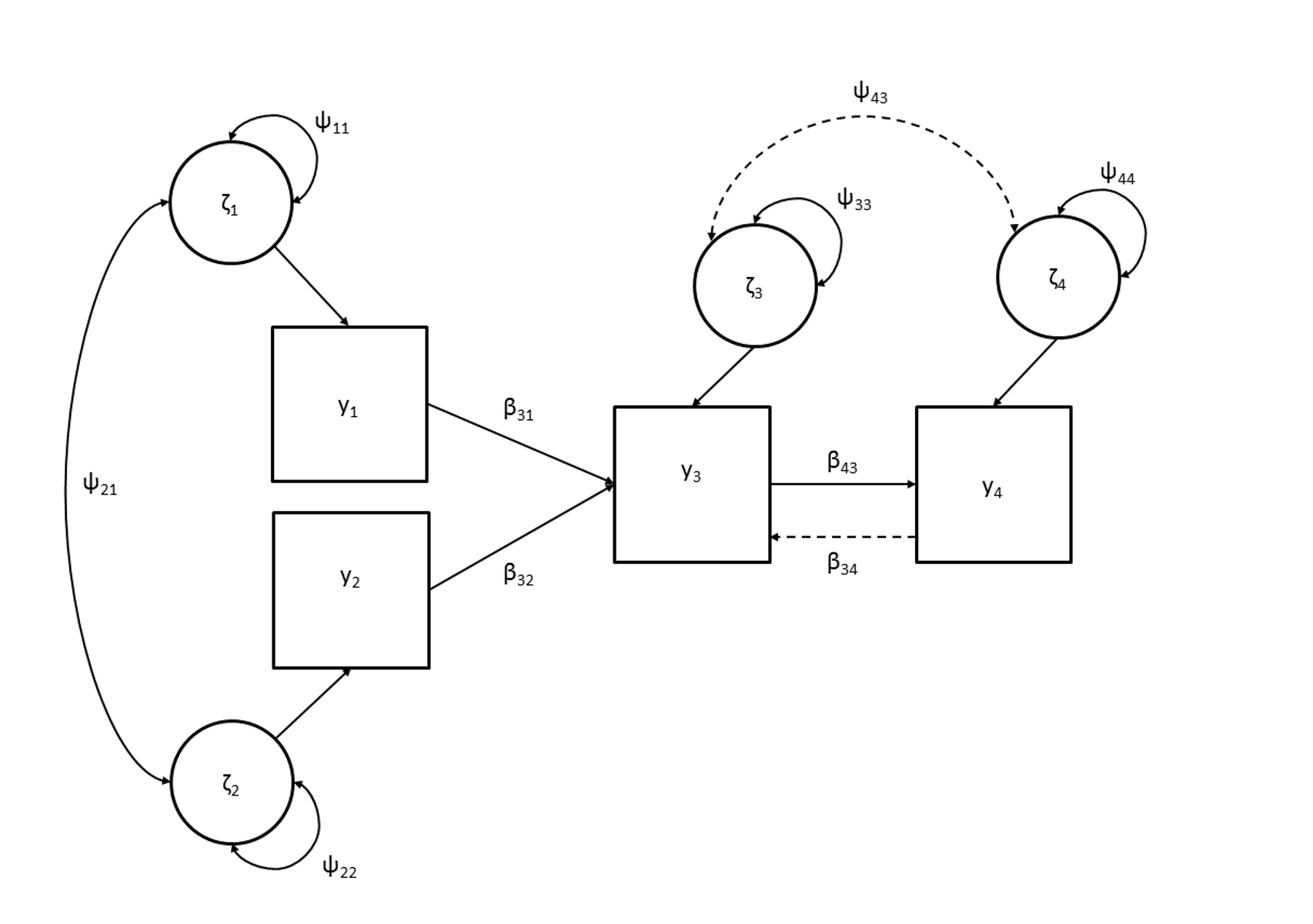
Figure 7.1: Path model for which identification is assessed in the situation when effects \(ψ_{43}\) (Model 1) and both \(ψ_{43}\) and \(ß_{34}\) (Model 2) are added.
## STEP 2: fit model to the covariance matrix from step 1

EmpiricalCheck <- '
            # regressions
            y4 ~ b43*y3
            y3 ~ b32*y2 + b31*y1

            # residual (co)variances
            y1 ~~ p11*y1
            y2 ~~ p22*y2
            y3 ~~ p33*y3
            y4 ~~ p44*y4
            y3 ~~ p43*y4

            # covariance exogenous variables
            y1 ~~ p21*y2
            '

EmpiricalCheckOut <- lavaan(EmpiricalCheck, sample.cov=SIGMA,
                     sample.nobs=100, likelihood = "wishart",
                     fixed.x=FALSE)

summary(EmpiricalCheckOut)
## lavaan 0.6-20.2318 ended normally after 20 iterations
##
## Estimator ML
## Optimization method NLMINB
## Number of model parameters 9
##
## Number of observations 100
##
## Model Test User Model:
##
## Test statistic 0.000
## Degrees of freedom 1
## P-value (Chi-square) 1.000
##
## Parameter Estimates:
##
## Standard errors Standard
## Information Expected
## Information saturated (h1) model Structured
##
## Regressions:
## Estimate Std.Err z-value P(>|z|)
## y4 ~
## y3 (b43) 0.500 0.097 5.150 0.000
## y3 ~
## y2 (b32) 0.500 0.085 5.906 0.000
## y1 (b31) 0.500 0.085 5.906 0.000
##
## Covariances:
## Estimate Std.Err z-value P(>|z|)
## .y4 ~~
## .y3 (p43) 0.500 0.119 4.194 0.000
## y2 ~~
## y1 (p21) 0.500 0.112 4.450 0.000
##
## Variances:
## Estimate Std.Err z-value P(>|z|)
## y1 (p11) 1.000 0.142 7.036 0.000
## y2 (p22) 1.000 0.142 7.036 0.000
## .y3 (p33) 0.800 0.114 7.036 0.000
## .y4 (p44) 0.700 0.139 5.035 0.000When you run the script for Model 1, you will notice that the parameter estimates are exactly equal to our chosen values from Step 1. Thus, this indicates that the model may be identified. As this empirical check is a necessary requirement for identification, but not sufficient, we are not completely sure that the model is truly identified.
In the next script we show the empirical check of Model 2, where we also add the effect from \(\mathrm{y}_4\) to \(\mathrm{y}_3\).
Script 7.2
## STEP 1: calculate the model implied covariance matrix

BETA <- matrix(c(0, 0, 0, 0,
             0, 0, 0, 0,
            .5,.5, 0,.5,
             0, 0,.5, 0),
             nrow=4,ncol=4,byrow=TRUE)

PSI <- matrix(c( 1,.5, 0, 0,
            .5, 1, 0, 0,
             0, 0,.8,.5,
             0, 0,.5,.7),
             nrow=4,ncol=4,byrow=TRUE)

IDEN <- diag(1,4,4)
SIGMA <- solve(IDEN-BETA) %*% PSI %*% t(solve(IDEN-BETA))

obsnames = c("y1","y2","y3","y4")
dimnames(SIGMA) <- list(obsnames,obsnames)


## STEP 2: fit model to the covariance matrix from step 1

EmpiricalCheck <- '
            # regressions
            y4 ~ b43*y3
            y3 ~ b32*y2 + b31*y1 + b34*y4

            # residual (co)variances
            y1 ~~ p11*y1
            y2 ~~ p22*y2
            y3 ~~ p33*y3
            y4 ~~ p44*y4
            y3 ~~ p43*y4

            # covariance exogenous variables
            y1 ~~ p21*y2
            '

EmpiricalCheckOut <- lavaan(EmpiricalCheck, sample.cov=SIGMA,
                     sample.nobs=100, likelihood = "wishart",
                     fixed.x=FALSE)
## Warning: lavaan->lav_model_vcov():
## Could not compute standard errors! The information matrix could not be
## inverted. This may be a symptom that the model is not identified.## lavaan 0.6-20.2318 ended normally after 21 iterations
##
## Estimator ML
## Optimization method NLMINB
## Number of model parameters 10
##
## Number of observations 100
##
## Model Test User Model:
##
## Test statistic 0.000
## Degrees of freedom 0
##
## Parameter Estimates:
##
## Standard errors Standard
## Information Expected
## Information saturated (h1) model Structured
##
## Regressions:
## Estimate Std.Err z-value P(>|z|)
## y4 ~
## y3 (b43) 0.500 NA
## y3 ~
## y2 (b32) 0.383 NA
## y1 (b31) 0.383 NA
## y4 (b34) 0.850 NA
##
## Covariances:
## Estimate Std.Err z-value P(>|z|)
## .y4 ~~
## .y3 (p43) 0.056 NA
## y2 ~~
## y1 (p21) 0.500 NA
##
## Variances:
## Estimate Std.Err z-value P(>|z|)
## y1 (p11) 1.000 NA
## y2 (p22) 1.000 NA
## .y3 (p33) 0.265 NA
## .y4 (p44) 0.700 NAThe output for the empirical check of Model 2 does not lead to the same parameter estimates as we used in Step 1. Therefore, we can be sure that this model is not identified.
Appendix
Algebraic assessment of identification using elements of \(\mathbf\Sigma_{\text{population}}\) and \(\mathbf\Sigma_{\text{model}}\)
\[\begin{equation} \beta_{31} = \frac{\sigma_{31}-\frac{\sigma_{32}-\beta_{31}\psi_{21}}{\psi_{22}}\psi_{21}}{\psi_{11}} \tag{7.9} \end{equation}\]
\[\begin{align} \beta_{31}\psi_{11} & = \sigma_{31}-\frac{\sigma_{32}\beta_{31}\psi_{21}}{\psi_{22}}\psi_{21} \ \ \ \ \ \ \ \ \ \ \ \ (7.09a)\\ \\ \beta_{31}\psi_{11}\psi_{22} & = \sigma_{31}\psi_{22} - (\sigma_{32}-\beta_{31} \psi_{21})\psi_{21} \ \ \ \ \ \ \ \ (7.09b)\\ \\ \beta_{31}\psi_{11}\psi_{22} & = \sigma_{31}\psi_{22} - \sigma_{32}\psi_{21} + \beta_{31}\psi^2_{21} \ \ \ \ \ \ \ \ (7.09c)\\ \\ \beta_{31}\psi_{11}\psi_{22} - \beta_{31}\psi^2_{21} & = \sigma_{31}\psi_{22} - \sigma_{32}\psi_{21} \ \ \ \ \ \ \ \ \ \ \ \ (7.09d)\\ \\ \beta_{31}(\psi_{11}\psi_{22} -\psi^2_{21}) & = \sigma_{31}\psi_{22} - \sigma_{32}\psi_{21} \ \ \ \ \ \ \ \ \ \ \ \ (7.09e) \end{align}\]
\[\begin{equation} \beta_{31} = \frac{\sigma_{31}\psi_{22}-\sigma_{32}\psi_{21}}{\psi_{11}\psi_{22}-{\psi_{21}}^2} \tag{7.10} \end{equation}\]
\[ \begin{align} \sigma_{33} = \dots \ \ \Longleftrightarrow \ \ \psi_{33} = \dots \ \ \ \ \ \ \ \ \ \ (7.13) \end{align} \] Substituting Equations (7.2), (7.3), (7.4), (7.11) and (7.13) into Equation (7.13) gives:
\[\begin{equation} \sigma_{33} = \frac{\sigma_{11}\sigma_{22}\sigma_{33}-2\sigma_{21}\sigma_{31}\sigma_{32}-\sigma_{11}\sigma^2_{32}-\sigma_{22}\sigma^2_{31}\sigma_{33}\sigma^2_{21}}{\sigma_{11}\sigma_{22}\sigma^2_{21}} \tag{7.14} \end{equation}\]
\[\begin{equation} \sigma_{41} = \dots 🡘 \beta_{43} = \frac{\sigma_{41}}{\beta_{31}\psi{11} + \beta_{32}\psi_{21}} \tag{7.15} \end{equation}\]
Substituting Equations (7.2), (7.4), (7.11) and (7.13) into Equation (7.15) gives:
\[\begin{equation} \beta_{43} = \frac{\sigma_{41}}{\sigma_{31}} \tag{7.16} \end{equation}\]
Although, to identify \(\beta_{43}\), we can also use:
\[\begin{equation} \sigma_{42} \Longleftrightarrow \beta_{43} = \frac{\sigma_{42}}{\beta_{31}\psi_{21} + \beta_{32}\psi_{22}} \tag{7.17} \end{equation}\]
Substituting Equations (7.2), (7.3), (7.11) and (7.12) into Equation (7.17) gives:
\[\begin{equation} \beta_{43} = \frac{\sigma_{42}}{\sigma_{31}} \tag{7.18} \end{equation}\]
So, now we already have two identifications of \(\beta_{43}\), and we can also use:
\[ \sigma_{43} = \dots \ \ \Longleftrightarrow \ \ \beta_{43} = \dots \ \ \ , \]
yielding:
\[\begin{equation} \beta_{43} = \frac{\sigma_{43}}{\sigma_{33}} \tag{7.19} \end{equation}\]
Equations (7.16), (7.17) and (7.19) show three identifications of \(\beta_{43}\).
\(\sigma_{44}\) identifies \(\psi_{44}\), through:
\[ \sigma_{44} = \dots \ \ \Longleftrightarrow \ \ \psi_{44} = \dots \ , \]
and substitution:
\[\begin{equation} \psi_{44} = \sigma_{44} - \sigma_{33}\beta^2_{43} \tag{7.20} \end{equation}\]
Which is identified after substituting either Equation (7.16), (7.18) or (7.19).