29 Fitting CFA models with multilevel data
In this chapter we introduce multilevel (two-level) factor models. These models will be relevant if one has obtained data with a nested structure, such as students nested in school classes, and the theoretical model involves latent variables. In Chapter 13, we introduced path models on observed variables with multilevel data. If constructs are operationalised with multiple indicators, these can be modeled using CFA. In a CFA with multilevel data, there are special considerations relating to measurement invariance and the interpretation of the common factor(s) at the different levels. We will illustrate the analysis of multilevel CFA using 6 indicators of teacher-student conflict. The items inquired after the amount of conflict students experiences with their teacher. An example item is: “I can be very angry at my teacher”. The items were scored on a 5-point Likert scale ranging from ‘definitely does not apply’ to ‘definitely does apply’. These items were answered by 800 students, on 44 independent teachers. So, the same teacher was the referent for about 20 students. For these data, it seems likely that the item responses from students that share a teacher will differ (some students experience more conflict than others with the same teacher), and that the average scores between teachers will vary (some teachers experience (on average) more conflict with their students than others).
Just as with multilevel path modeling, the item responses can be decomposed in a within-cluster and between-cluster part. The item scores from subject i in cluster j are decomposed into means (\(\mu_j\)), and individual deviations from the cluster means (\(\eta_{ij}\)):
\[\begin{align} \mathrm{y}_{ij} &= \mu_j + (\mathrm{y}_{ij} - \mu_j) \\ &= \mu_j + \eta_{ij} \end{align}\]
where \(\mu_j\) and \(\eta_{ij}\) are independent. In the example of teacher-student conflict, a person’s within-component of an item, \(\eta_{ij}\), reflects the person’s score on that conflict item deviates from the average scores of that item across all students who shared the specific teacher (\(\mu_j\)). The \(\mu_j\) component thus reflects how the teacher’s item score (obtained by averaging the item scores of the students) deviates from the overall mean item score.
Just as with multilevel path analysis, the overall covariances of \(y_{ij}\) (\(\Sigma_{total}\)) can be written as the sum of the covariances of these two components:
\[\begin{align} \mathbf\Sigma_\text{total} &= \text{COV}(\mu_j, \mu_j) + \text{COV}(\eta_{ij}, \eta_{ij}) \\ &= \mathbf\Sigma_\text{between} + \mathbf\Sigma_\text{within} \\ &= \mathbf\Sigma_\text{B} + \mathbf\Sigma_\text{W} \end{align}\]
29.1 Intraclass correlations of observed variables
Intraclass correlations (ICCs) indicate what proportion of a variable’s total variance exists at Level 2. Script 29.1 shows how to obtain the ICCs of the conflict items using lavaan.the file "conflict.dat" contains the item scores of the students (multilevel models require the analysis of raw data).
Script 29.1
library(lavaan)
data <- read.table("demoData/conflict.dat")
names(data) <- c("teacher",paste0("v",1:6))

head(data)
## teacher v1 v2 v3 v4 v5 v6
## 1 41 1 1 1 1 1 1
## 2 41 1 4 1 1 1 5
## 3 41 1 1 1 1 1 1
## 4 41 1 1 1 1 1 4
## 5 41 1 1 2 1 1 1
## 6 41 1 1 1 1 1 1modelsat <- '
level: 1
v1 ~~ v2 + v3 + v4 + v5 + v6
v2 ~~ v3 + v4 + v5 + v6
v3 ~~ v4 + v5 + v6
v4 ~~ v5 + v6
v5 ~~ v6
level: 2
v1 ~~ v2 + v3 + v4 + v5 + v6
v2 ~~ v3 + v4 + v5 + v6
v3 ~~ v4 + v5 + v6
v4 ~~ v5 + v6
v5 ~~ v6
v1 ~ 1
v2 ~ 1
v3 ~ 1
v4 ~ 1
v5 ~ 1
v6 ~ 1
'
fitsat <- lavaan(modelsat, data = data, cluster = "teacher", auto.var = TRUE)
# extract covariance matrices to calculate ICCs manually
Sigma_w <- lavInspect(fitsat, "sampstat")$within$cov
Sigma_b <- lavInspect(fitsat, "sampstat")$teacher$cov
ICC <- diag(Sigma_b/(Sigma_b + Sigma_w))
round(ICC,3)## v1 v2 v3 v4 v5 v6
## 0.072 0.072 0.042 0.044 0.046 0.232## v1 v2 v3 v4 v5 v6
## 0.072 0.072 0.042 0.044 0.046 0.23229.2 Multilevel structure as a nuisance: Correcting for the dependency
If you add the argument cluster = “clustervariable”, then lavaan will report cluster-robust \(SE\)s (Williams, 2000) and a corrected test statistic. This would be an acceptable approach when your hypotheses are only about Level 1 processes, and you just want to correct for the nested data. In this approach, the factor model is effectively fit to \(\mathbf\Sigma_\text{total}\). If a research question involves hypotheses at Level 1 and Level 2, or it involves latent variables at Level 2, the one should take the two-level approach.
29.3 Two-level factor models
In the within/between formulation (Muthén, 1990, 1994; Schmidt, 1969), one can postulate separate models for \(\mathbf\Sigma_\text{B}\) and \(\mathbf\Sigma_\text{W}\). Technically, these models can be completely different (one could even fit a path model to one level and a factor model to the other level). However, to obtain an appropriate interpretation of common factors at different levels, one often needs some constraints across levels. In our conflict example, we could name the common factor “teacher-student conflict”.
Similar to the decomposition of the observed variables into a within-cluster and a between-cluster component, one could imagine decomposing the (unobserved) common factor scores:
\[\begin{align} \xi_{ij} &= \kappa_j + (\xi_{ij} - \kappa_j) \\ &= \kappa_j + \gamma_{ij} \end{align}\]
In this decomposition \(\kappa_j\) represents the cluster averages on the common factor, and \(\gamma_{ij}\) represents the individual deviations from the cluster average on the common factor. For such an interpretation, the factor loadings relating the common factor to the indicators should be invariant across levels. If the common factor is the only variable that differs at both levels, there will not be residual factors (and residual variance) at the between level. This kind of model is called the variance components factor model by Rabe, Hesketh & Skrondal (2004). Note that this variance components factor model represents the situation in which all observed differences in the cluster means of the indicators results from cluster mean differences in the common factor. In other words, observed differences between clusters are not the result of differences in measurement parameters (factor loadings, intercepts, or residual variances), which corresponds to the definition of measurement invariance. Indeed, the variance components factor model represents a model with strong factorial invariance (or equivalently, scalar invariance) across clusters. If strong factorial invariance across clusters holds, then the models for \(\mathbf\Sigma_\text{within}\) an \(\mathbf\Sigma_\text{between}\) are:
\[\begin{align} \mathbf\Sigma_\text{W} &= \mathbf\Lambda \mathbf\Phi_\text{W} \mathbf\Lambda^\intercal + \mathbf\Theta_\text{W} \\ \mathbf\Sigma_\text{B} &= \mathbf\Lambda \mathbf\Phi_\text{B} \mathbf\Lambda^\intercal \\ \end{align}\]
If indicator intercepts are not equal across clusters, but factor loadings are (so weak factorial invariance/metric invariance holds), then the intercept differences across clusters will will appear as residual variance at the between-level:
\[\begin{align} \mathbf\Sigma_\text{W} &= \mathbf\Lambda \mathbf\Phi_\text{W} \mathbf\Lambda^\intercal + \mathbf\Theta_\text{W} \\ \mathbf\Sigma_\text{B} &= \mathbf\Lambda \mathbf\Phi_\text{B} \mathbf\Lambda^\intercal + \mathbf\Theta_\text{B}\\ \end{align}\]
In such a case, the common factor at the two levels still represents the within- and between components of the same common factor.
If in addition the factor loadings are not equal, so that weak factorial invariance (metric) invariance across clusters does not hold, then this will also lead to increased residual variance at the between level, and in addition the factor loadings may become unequal across levels (Jak, Oort & Dolan, 2013; Muthén & Asparouhov, 2018). If factor loadings are unequal across levels, the interpretation of the common factor at the two levels becomes very complicated, as they do not longer represent the within- and between components of the same latent variable (Mehta & Neale, 2005). Moreover, it would mean that the common factor has a different interpretation in each cluster. The between-level part of the model then reflects a model for cluster differences in different latent variables (Jak & Jorgensen, 2017).
Script 29.2 fits the multilevel factor model to the six conflict indicators, in which there is one factor underlying the indicator scores. Below you can find a graphical display of the model.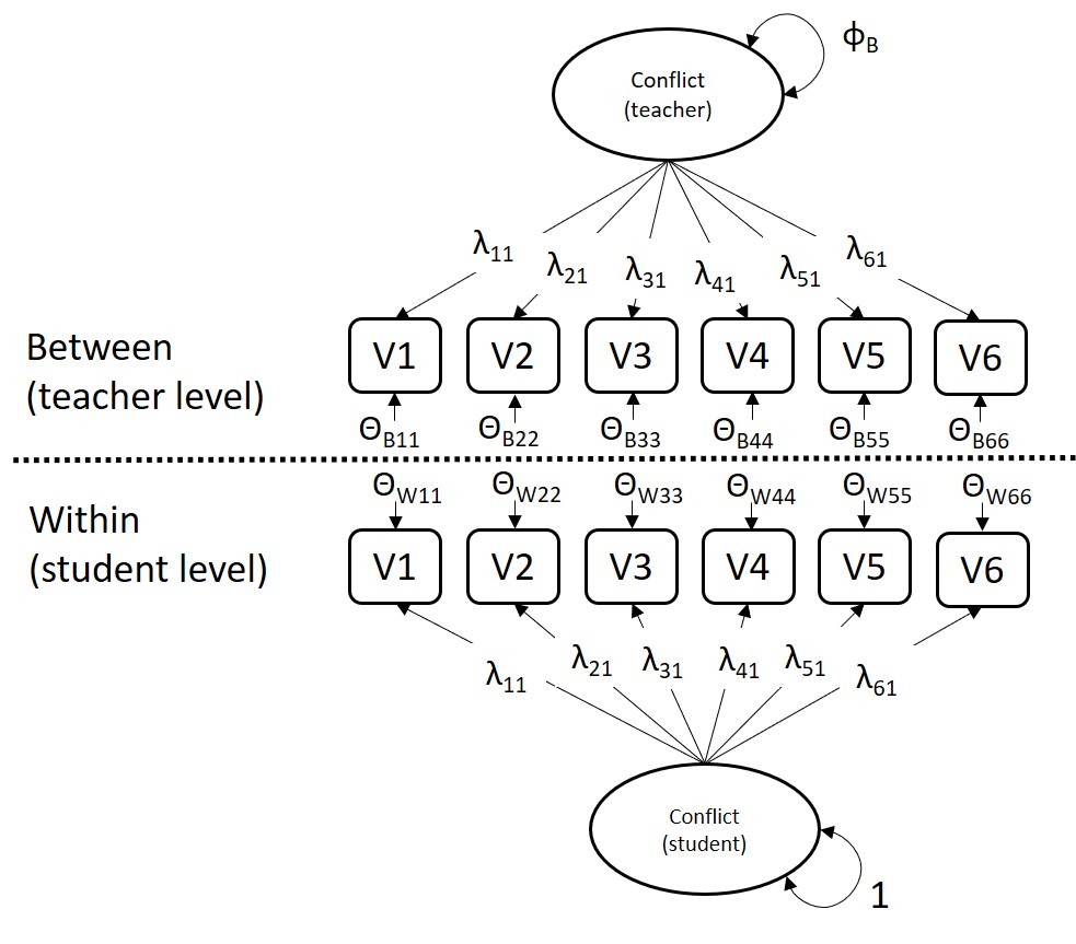
Figure 29.1: A two-level factor model on six conflict items.
The factor loadings are constrained to be equal across levels by providing the same labels to the parameters across levels. Because these equality constraints already provide a scale to the between-level common factor, the factor variance at the between level is freely estimated, while the factor variance at the within level is fixed at one (this could also be specified the other way around). In this model the residual variances at the between level are freely estimated.
Script 29.2
# Fit two-level factor model with equal factor loadings across levels

model1 <-  '
  level: 1
  # factor loadings
  conflict =~ L11*v1 + L21*v2 + L31*v3 + L41*v4 + L51*v5 + L61*v6

  # factor variance fixed at 1
  conflict ~~ 1*conflict

  # residual variances
  v1 ~~ v1
  v2 ~~ v2
  v3 ~~ v3
  v4 ~~ v4
  v5 ~~ v5
  v6 ~~ v6

level: 2
  # factor loadings
  conflict =~ L11*v1 + L21*v2 + L31*v3 + L41*v4 + L51*v5 + L61*v6

  # factor variance free
  conflict ~~ phi_b*conflict

  # residual variances
  v1 ~~ th1*v1
  v2 ~~ th2*v2
  v3 ~~ th3*v3
  v4 ~~ th4*v4
  v5 ~~ th5*v5
  v6 ~~ th6*v6

  # intercepts
  v1 ~ 1
  v2 ~ 1
  v3 ~ 1
  v4 ~ 1
  v5 ~ 1
  v6 ~ 1
'

fit1 <- lavaan(model1, data = data, cluster = "teacher")

summary(fit1, fit = TRUE)
## lavaan 0.6-20.2318 ended normally after 59 iterations
##
## Estimator ML
## Optimization method NLMINB
## Number of model parameters 31
## Number of equality constraints 6
##
## Number of observations 800
## Number of clusters [teacher] 44
##
## Model Test User Model:
##
## Test statistic 49.694
## Degrees of freedom 23
## P-value (Chi-square) 0.001
##
## Model Test Baseline Model:
##
## Test statistic 1209.905
## Degrees of freedom 30
## P-value 0.000
##
## User Model versus Baseline Model:
##
## Comparative Fit Index (CFI) 0.977
## Tucker-Lewis Index (TLI) 0.970
##
## Loglikelihood and Information Criteria:
##
## Loglikelihood user model (H0) -5096.885
## Loglikelihood unrestricted model (H1) -5072.039
##
## Akaike (AIC) 10243.771
## Bayesian (BIC) 10360.886
## Sample-size adjusted Bayesian (SABIC) 10281.497
##
## Root Mean Square Error of Approximation:
##
## RMSEA 0.038
## 90 Percent confidence interval - lower 0.023
## 90 Percent confidence interval - upper 0.053
## P-value H_0: RMSEA <= 0.050 0.907
## P-value H_0: RMSEA >= 0.080 0.000
##
## Standardized Root Mean Square Residual (corr metric):
##
## SRMR (within covariance matrix) 0.024
## SRMR (between covariance matrix) 0.188
##
## Parameter Estimates:
##
## Standard errors Standard
## Information Observed
## Observed information based on Hessian
##
##
## Level 1 [within]:
##
## Latent Variables:
## Estimate Std.Err z-value P(>|z|)
## conflict =~
## v1 (L11) 0.398 0.019 21.149 0.000
## v2 (L21) 0.402 0.022 18.073 0.000
## v3 (L31) 0.485 0.027 17.728 0.000
## v4 (L41) 0.544 0.037 14.739 0.000
## v5 (L51) 0.458 0.028 16.487 0.000
## v6 (L61) 0.572 0.033 17.233 0.000
##
## Variances:
## Estimate Std.Err z-value P(>|z|)
## conflict 1.000
## .v1 0.148 0.011 14.027 0.000
## .v2 0.258 0.016 16.467 0.000
## .v3 0.379 0.023 16.278 0.000
## .v4 0.731 0.042 17.357 0.000
## .v5 0.432 0.025 17.027 0.000
## .v6 0.516 0.032 16.355 0.000
##
##
## Level 2 [teacher]:
##
## Latent Variables:
## Estimate Std.Err z-value P(>|z|)
## conflict =~
## v1 (L11) 0.398 0.019 21.149 0.000
## v2 (L21) 0.402 0.022 18.073 0.000
## v3 (L31) 0.485 0.027 17.728 0.000
## v4 (L41) 0.544 0.037 14.739 0.000
## v5 (L51) 0.458 0.028 16.487 0.000
## v6 (L61) 0.572 0.033 17.233 0.000
##
## Intercepts:
## Estimate Std.Err z-value P(>|z|)
## .v1 1.196 0.032 37.273 0.000
## .v2 1.238 0.033 37.195 0.000
## .v3 1.418 0.042 34.037 0.000
## .v4 1.713 0.058 29.645 0.000
## .v5 1.349 0.040 33.781 0.000
## .v6 1.605 0.070 22.948 0.000
##
## Variances:
## Estimate Std.Err z-value P(>|z|)
## conflct (ph_b) 0.152 0.051 2.984 0.003
## .v1 (th1) 0.002 0.003 0.829 0.407
## .v2 (th2) -0.001 0.004 -0.250 0.803
## .v3 (th3) 0.004 0.006 0.654 0.513
## .v4 (th4) 0.039 0.018 2.205 0.027
## .v5 (th5) 0.001 0.006 0.108 0.914
## .v6 (th6) 0.110 0.032 3.460 0.001The overall fit of this model is acceptable. Next, we evaluate whether the residual variances at the between level can be constrained to zero, which would represent strong factorial invariance across clusters.
fixtheta <-
'th1 == 0
 th2 == 0
 th3 == 0
 th4 == 0
 th5 == 0
 th6 == 0'

fit2 <- lavaan(c(model1,fixtheta), data = data, cluster = "teacher")

anova(fit1,fit2)
##
## Chi-Squared Difference Test
##
## Df AIC BIC Chisq Chisq diff RMSEA Df diff Pr(>Chisq)
## fit1 23 10244 10361 49.694
## fit2 29 10316 10405 133.573 83.879 0.12738 6 5.634e-16 ***
## ---
## Signif. codes: 0 '***' 0.001 '**' 0.01 '*' 0.05 '.' 0.1 ' ' 1The fit results show that constraining the residual variances to zero leads to significantly worse model fit according to the chi-square difference test. Moreover, the AIC is lower for model 1. Therefore, we would continue with model 1.
29.4 Intraclass correlations of common factors
In a model in which factor loadings are equal across levels, one can calculate the intraclass correlation of the common factor(s) (Mehta & Neale, 2005) using:
\[\begin{align} \text{ICC} &= \frac{\mathbf\Phi_\text{B}}{\mathbf\Phi_\text{B} + \mathbf\Phi_\text{W}}\\ \end{align}\]
These ICCs represent the proportion of a common factor’s total variance that exists at Level 2. For the conflict factor, the common factor variance at the within level is fixed at 1 for identification, and the common factor variance at the between level is estimated as 0.152, so the intraclass correlation of the common factor equals 0.152 / ( 0.152 + 1) = 0.132.
29.5 Climate and contextual between-level latent variables
Researchers frequently use the responses of individuals in clusters to measure constructs at the cluster level. For example, in educational research, student evaluations may be used to measure the teaching quality of instructors. in other fields, patient reports may be used to evaluate social skills of therapists, and residents’ ratings may be used to evaluate neighborhood safety. In these three examples the target construct is something that (in theory) only varies at the cluster level; the individuals within one cluster all share the same instructor, therapist, or neighborhood.
A contrasting type of cluster-level constructs can be defined as constructs that theoretically differ across individuals within the same cluster. Examples are reading skills of students in a classroom, depressive symptoms of individual patients of a therapist, and number of years that individuals live in a particular neighborhood. Although the target construct here is defined at the individual level, it is quite likely that the averages across clusters will also vary due to cluster-level factors. For instance, the average reading skills of students in different classrooms may differ due to differences of teaching styles or years of teaching experience across classrooms, the average amount of depressive symptoms of patients may differ across therapists due to differences in therapists’ approaches, and some neighborhoods may have a higher turnaround of residence than other neighborhoods due to differences in local council policies and amenities.
In the terminology of Marsh et al. (2012), if the referent of the item is the individual (e.g., “I like going to school”), then the cluster-level variable represents a contextual construct. If the referent of the item is the cluster (e.g., “My school is fun to go to”), then the cluster-aggregate represents a climate construct. The distinction between these types of constructs is more a theoretical one than a statistical one, because the same factor model (with equal factor loadings across levels) applies for both types of constructs. Marsh et al. (2012) call this factor model the doubly latent model. ‘Doubly latent’ in this context refers to using multiple indicators to measure a common factor, and decomposing the observed indicators into latent within- and between parts.
29.6 Full SEM with multilevel data
In this chapter we only discussed CFA, and in Chapter 13 we only discussed path models on observed variables with multilevel data. One can also fit path models n latent variables (full SEM) with multilevel data. Similar to single level analysis, this would involve two steps. First one would establish a good measurement model using CFA, and in a second step one could specify a path model on the common factors. In practice, the number of clusters is often relatively small. In our example, we have measurements about only 44 teachers. The sample size at the between-level is thus 44, which is very small. With such small samples it is not possible to evaluate very complex models with many parameters, even in single level analysis. Therefore, the general advice is to keep the between-level model as simple as possible, and to collect data from many clusters if the research question involves between-level variables. One alternative option to test path models on latent variables would be using simple regression analysis on factor scores (see Devlieger & Rosseel, 2020).
References
Devlieger, I., & Rosseel, Y. (2020). Multilevel factor score regression. Multivariate behavioral research, 55(4), 600-624.
Jak, S. & Jorgensen, T.D. (2017). Relating measurement invariance, cross-level invariance, and multilevel reliability. Frontiers in Psychology, 8, 1640.
Jak, S., Oort, F.J. & Dolan, C.V. (2013). A test for cluster bias: Detecting violations of measurement invariance across clusters in multilevel data. Structural Equation Modeling, 20, 265-282.
Marsh, H. W., Lüdtke, O., Robitzsch, A., Trautwein, U., Asparouhov, T., Muthén, B., & Nagengast, B. (2009). Doubly-latent models of school contextual effects: Integrating multilevel and structural equation approaches to control measurement and sampling error. Multivariate Behavioral Research, 44(6), 764-802.
Mehta, P. D., & Neale, M. C. (2005). People are variables too: multilevel structural equations modeling. Psychological methods, 10(3), 259.
Muthén, B.O. (1990). Mean and covariance structure analysis of hierarchical data. Los Angeles, CA: UCLA.
Muthén, B.O. (1994). Multilevel covariance structure analysis. Sociological Methods & Research, 22(3), 376–398. https://doi.org/10.1177%2F0049124194022003006
Muthén, B.O., & Asparouhov, T. (2018). Recent methods for the study of measurement invariance with many groups: Alignment and random effects. Sociological Methods & Research, 47(4), 637-664.
Rabe-Hesketh, S., Skrondal, A., & Pickles, A. (2004). Generalized multilevel structural equation modeling. Psychometrika, 69(2), 167-190.
Williams, R. L. (2000). A note on robust variance estimation for cluster‐correlated data. Biometrics, 56(2), 645–646. https://doi.org/10.1111/j.0006-341X.2000.00645.x
Schmidt, W. H. (1969). Covariance structure analysis of the multivariate random effects model [Doctoral dissertation]. University of Chicago, Department of Education.