5 Direct, Indirect, and Total Effects
In the path model from our illustrative example (see Figure 5.1), there is no arrow pointing from Parental Anxiety (PA) to Child anxiety (CA). This does not mean that the model implies that there is no effect of PA on CA. The effect runs through Parental Overcontrol (PO). PA has a direct effect on PO, which in turn has a direct effect on CA. PA thus has an indirect effect on CA, reflecting that the effect of PA on CA is mediated by PO. The size of the indirect effect equals the product of the direct effects that constitute the indirect effect. So, in this example, the indirect effect of PA on CA through PO is equal to .187 (\(β_{31}\)) times .072 (\(β_{43}\)) = .013. Note that it makes sense that the indirect effect equals the product of the direct effects. Holding PP constant, if PA increases with one point, PO is expected to increase with .187 point. If PO increases with 1 point, CA is expected to increase with .072 point. So if PO increases with .187 points instead of 1 point, CA is expected to increase with \(.187 \times .072 = .013\) points. Similarly, the indirect effect of Parental Perfectionism (PP) on CA is \(.210 \times .072 = .015\), indicating that 1 point increase in PP is expected to result in .015 point increase of CA.
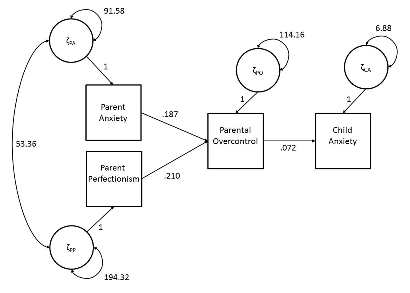
Figure 5.1: Full Mediation Model.
If an effect of one variable on the other is only indirect, this reflects full mediation. Very often, there is also a direct effect next to the indirect effect, reflecting that the effect is not fully mediated, but partially mediated. Figure 5.2 shows the path model example of the partial mediation model (i.e., with direct effects of PA and PP on CA) and the associated parameter estimates.
The direct effect of PA on CA is .091. This is the part of the total effect that is not mediated by PO. The total effect of PA on CA is the sum of the indirect effect(s) and the direct effect: \(.091 + .187 \times .058 = .102\). Total effects thus are the sum of all indirect and direct effects of one variable on another. This is an example of consistent mediation, i.e., the direct effect and the indirect have the same sign (they are both positive in this case). It could also be that there is inconsistent mediation, where the direct effect and indirect have opposite signs. In our example, there is inconsistent mediation of the effect of PP on CA as the direct effect is negative while the indirect effect is positive. Inconsistent mediation could therefore lead to the situation in which the direct effect and indirect effect cancel each other out.
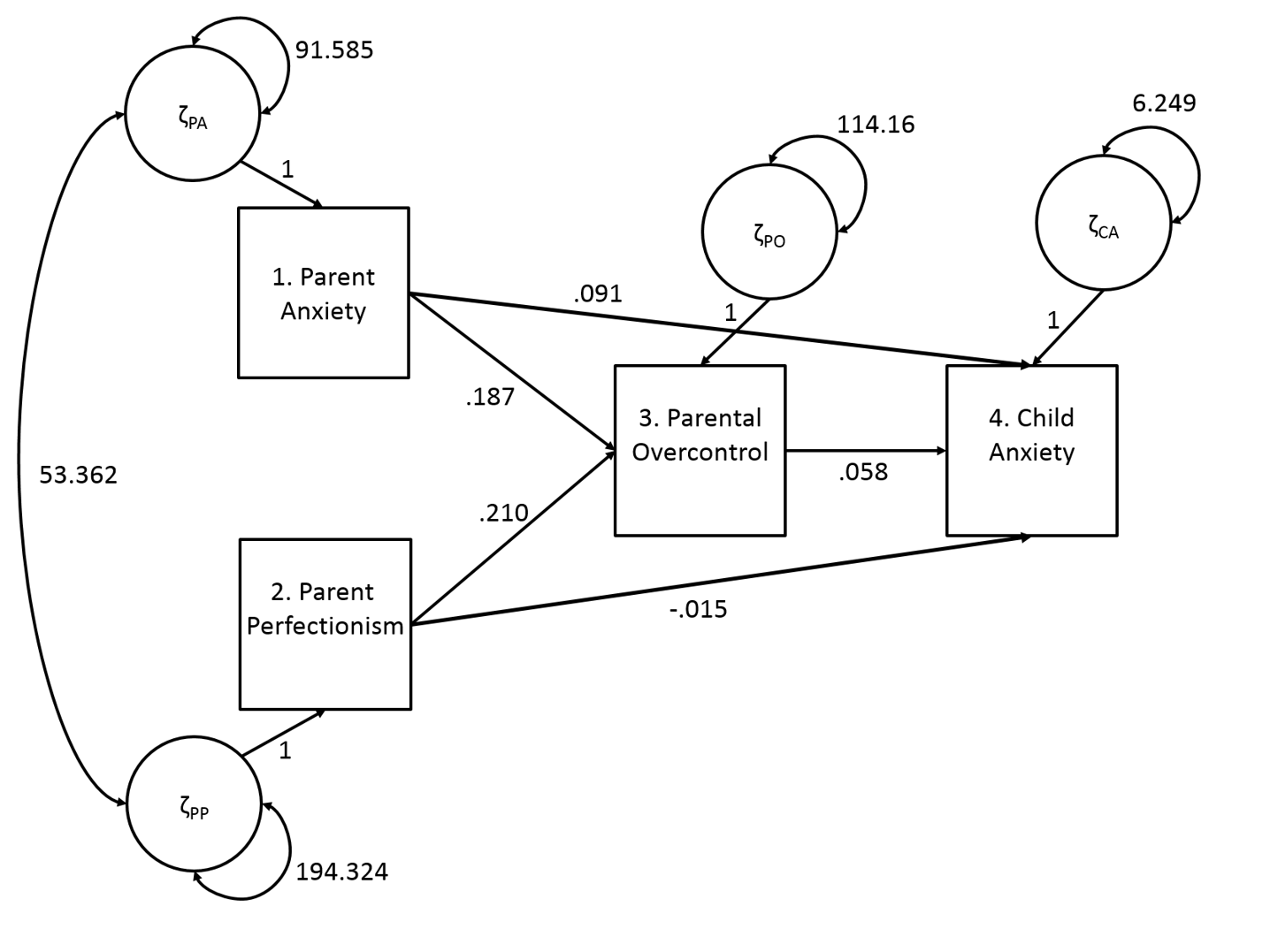
Figure 5.2: Partial Mediation Model.
5.1 Testing significance of indirect effects
Testing the significance of indirect effects can be done in the same way as for testing the significance of direct effects, using the standard error (\(SE\)) of the estimated effect. However, because the indirect effect is the product of two direct effects, the sampling distribution of the estimated indirect effects are complex and the associated SE’s are unknown. Sobel (1982) suggested to use the so-called delta-method (Rao, 1973; Oehlert, 1992) to obtain an approximation of the standard errors for unstandardized indirect effects. Suppose a is the effect of the predictor on the mediator, and b is the effect of the mediator on the outcome variable, then the estimated standard error for the indirect effect \(ab\) is:
\[\begin{equation} SE_{ab} = \sqrt{b^2SE^2_a + a^2SE^2_b} \tag{5.1} \end{equation}\]
When the sample size is large, the ratio \(ab / SE_{ab}\) can be used as the \(z\) test of the unstandardized indirect effect. This is called the Sobel-test (Sobel, 1982). With small samples, if the raw data is available, it is preferred to bootstrap confidence intervals around indirect effects (Preacher & Hayes, 2008). If raw data is not available, bootstrapping is not an option. In this case one could use likelihood based confidence intervals (Cheung, 2008). Likelihood based confidence intervals are not available in lavaan. lavaan will provide standard errors based on the delta-method. Table 1 gives an overview of the direct, indirect and total effects of PA and PP on CA. In our example, none of the indirect effects are significant.
Table 1. Direct, total indirect and total effects on Child Anxiety with standard errors, z-values and p-values and standardized values for the model from Figure 2.
| Parameter | Estimate | SE | Z-value | p(>|z|) | LB 95%CI | UB 95%CI | Std. |
|---|---|---|---|---|---|---|---|
| Effects from PA on CA | |||||||
| Direct | .091 | .033 | 2.771 | .006 | .027 | .155 | .317 |
| Total indirect | .011 | .009 | 1.148 | .251 | -.008 | .029 | .038 |
| Total | .102 | .033 | 3.047 | .002 | .036 | .168 | .355 |
| Effects from PP on CA | |||||||
| Direct | -.015 | .023 | -.635 | .525 | -.060 | .030 | -.074 |
| Total indirect | .012 | .008 | 1.552 | .121 | -.003 | .028 | .062 |
| Total | -.002 | .023 | -.103 | .918 | -.047 | .043 | -.012 |
5.2 Higher order indirect effects
In our example there are only two indirect effects, but there may be more complex indirect effects. Consider for example the model that was hypothesized by Affrunti and Woodruff-Borden (2014) in Figure 5.3.
In the model of Figure 5.3, there are two indirect effects from PA on CA. One path goes from PA to PO and then from PO to CA, and is equal to \(β_{31} \times β_{43}\). The other indirect effect goes from PA to PP, from PP to PO, and from PO to CA, and is calculated by \(β_{21} \times β_{32} \times β_{43}\). Because this effect is build up of three direct effects, this is called a third order effect. The sum of all specific indirect effects is the total indirect effect. The total effect of PA on CA equals the sum of all indirect effects plus the direct effect (\(β_{41}\)). This model also contains an indirect effect of PA on PO, which equals \(β_{21} \times β_{32}\).
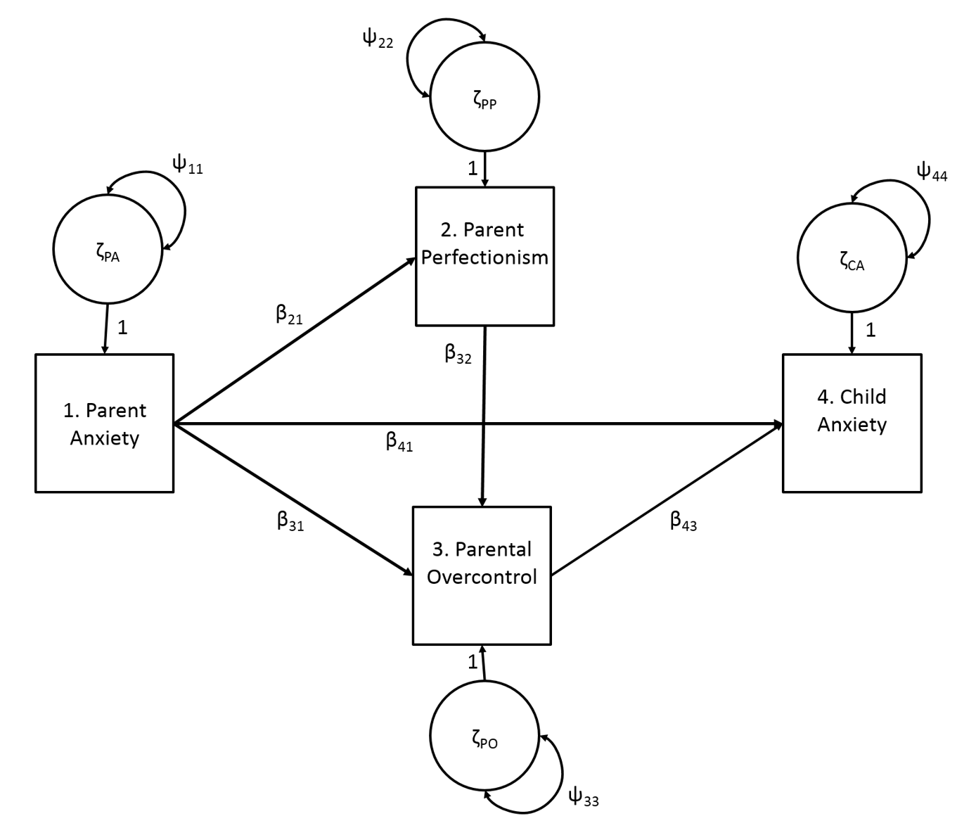
Figure 5.3: The hypothesized model of Affrunti and Woodruff-Borden (2014).
Judging the significance of higher order indirect effects can also be done using the delta-method and Sobel test described earlier, but the calculations quickly become more difficult. For example, the standard error of indirect effect abc can be calculated using \(SE_{abc} = SE_{ab} \times SE_{c}\) using Equation (5.1). lavaan will provide standard errors based on the delta-method for all requested functions of parameters.
Table 2 shows a decomposition of effects of PA on PO and of PA on CA. As can be seen in Table 2, none of the individual indirect effects, or the total indirect effects in the model are significantly larger than zero. The unstandardized total effect of PA on CA is estimated to be .101, and is statistically significant at \(α\) = .05. As can be seen, the total effect can be attributed to the direct effect of PA on CA. The total effect of PA on PO is also statistically significant, although both the direct and the total indirect effects are not significant individually. Their combined effect leads to a total effect that is large enough to lead to statistical significance.
Table 2. Direct, total indirect and total effects on CA and PO with standard errors, z-values and p-values and standardized values for path model from Figure 3.
| Parameter | Estimate | SE | Z-value | p(>|z|) | LB 95%CI | UB 95%CI | Std. |
|---|---|---|---|---|---|---|---|
| Effects from PA on CA | |||||||
| Direct | .084 | .031 | 2.271 | .007 | .023 | .144 | .292 |
| Indirect via PP and PO | .007 | .005 | 1.409 | .159 | -.003 | .016 | .023 |
| Indirect via PO | .010 | .009 | 1.133 | .257 | -.007 | .028 | .035 |
| Total indirect | .017 | .011 | 1.563 | .118 | -.004 | .038 | .058 |
| Total | .101 | .031 | 3.279 | .001 | .040 | .161 | .350 |
| Effects from PA on PO | |||||||
| Direct | .187 | .139 | 1.350 | .177 | -.085 | .459 | .157 |
| Indirect via PP | .123 | .064 | 1.913 | .056 | -.003 | .248 | .103 |
| Total indirect | .123 | .064 | 1.913 | .056 | -.003 | .248 | .103 |
| Total | .310 | .131 | 2.363 | .018 | .053 | .567 | .260 |
After fitting a model, the estimated direct effects can be used to calculate the specific indirect effects, the total indirect effects and the total effects by hand. However, this is a tedious job. Therefore, it is often more attractive to use matrix algebra to obtain the indirect and total effects.
5.3 Using matrix algebra to calculate total, total indirect and specific indirect effects
Instead of calculating all total effects by hand, one can use the model matrix \(\mathbf{B}\) to calculate the total effects. In recursive models, the total effects in matrix \(\mathbf{T}\) are given by:
\[\begin{equation} \mathbf{T}=\sum _{k=1}^{p-1}{\mathbf{B}}^{k} \tag{5.2} \end{equation}\]
where \(p\) is the number of variables. Thus, the total effects are calculated using the sum of powers of the matrix with regression coefficients (\(\mathbf{B}\)), where the highest number of powers (\(k\)) is equal to the number of variables minus one (\(p - 1\)). For example, with four variables the total effects can be calculated using: \(\mathbf{T} = \mathbf{B}^1 + \mathbf{B}^2 + \mathbf{B}^3\). As \(\mathbf{B}^1 = \mathbf{B}\), the total effects can be decomposed into matrix B that contains all direct effects, and the sum of the powers of the \(\mathbf{B}\) matrix that contain all indirect effects. Thus, the matrix with all indirect effects can be calculated by \(\mathbf{T} - \mathbf{B}\).
In the anxiety example path model with higher order indirect effects the \(\mathbf{B}\) matrix is:
\[ \mathbf{B}^1 = \begin{bmatrix} 0 &0 &0&0 \\ \beta_{21} & 0 & 0&0\\ \beta_{31} & \beta_{32} & 0&0 \\ \beta_{41} & 0 & \beta_{43} & 0 \end{bmatrix}. \]
which contains all direct effects (i.e., first-order effects). Multiplying matrix \(\mathbf{B}\) with itself gives \(\mathbf{B}^2\), which contains all second-order indirect effects:
\[ \mathbf{B}^2 = \begin{bmatrix} 0 &0 &0&0 \\ 0 & 0 & 0&0\\ \beta_{21}\beta_{32} & 0 & 0&0 \\ \beta_{31}\beta_{43} & \beta_{32}\beta_{43} & 0 & 0 \end{bmatrix}. \]
Multiplying matrix \(\mathbf{B}\) with itself three times gives the third-order indirect effects:
\[ \mathbf{B}^3 = \begin{bmatrix} 0 &0 &0&0 \\ 0 & 0 & 0&0\\ 0 & 0 & 0&0 \\ \beta_{21}\beta_{32}\beta_{43} & 0 & 0 & 0 \end{bmatrix}. \]
If we would continue and calculate \(\mathbf{B}^4\) we will see that it contains only zeros (indicating that there cannot exist fourth-order indirect effects in the model with four variables). Similarly, if we would calculate the matrices of indirect effects for the example in Figure 5.2, matrix \(\mathbf{B}^3\) would already be zero, because there are no third or higher order effects in this model. The sum of the direct effects and the indirect effects is equal to the total effects.
For nonrecursive models (discussed in a later chapter), Equation (5.2) can often still be used to calculate total effects, but it is not necessarily adequate. That is, the number of times that the power of the matrix with regression coefficients has to be calculated (and summed) is not defined. The total effects are only defined when the power of the matrix with regression coefficients (\(\mathbf{B}^k\)) converges to zero.
5.4 Calculating total, total indirect and specific indirect effects using lavaan output
We will use the output of the anxiety model to compute a matrix that contains the total effects (\(\mathbf{T}\)), a matrix that contains the total indirect effects (\(\mathbf{U}\)) and illustrate the calculation of a specific indirect effects (I1).
In recursive models, matrix \(\mathbf{T}\) is calculated by addition of matrix B with multiplications of matrix \(\mathbf{B}\), as often as the number of variables minus one. So, if there are 4 observed variables, the expression for \(\mathbf{T}\) stops after \(\mathbf{B}\) is multiplied with itself 3 times. \(\mathbf{T}\) contains the total effects.
Estimates <- lavInspect(AWmodelOut, "est")
B <- Estimates$beta[obsnames, obsnames]
Tot <- B + B %*% B + B %*% B %*% B
Matrix \(\mathbf{U}\) is calculated as the matrix with total effects, minus the matrix with direct effects. The result is a matrix with the total indirect effects. Please notice that if there are multiple indirect effects between two variables, matrix \(\mathbf{U}\) has the sum of the indirect effects.
A single indirect effect is calculated by multiplying specific elements from matrix \(\mathbf{B}\). For example, B[3,1] selects the element in row 3, column 1 from the \(\mathbf{B}\) matrix, and this element is multiplied with element B[4,3]. This is the indirect effect of Parental anxiety on Child anxiety via Overcontrol (see Figure 5.1). We gave this effect the name I1, because you may want to calculate more indirect effects, which could then be named I2, I3, I4 etc.
The resulting matrices are shown by asking for the result:
##             parent_anx    perfect overcontrol child_anx
## parent_anx  0.00000000 0.00000000  0.00000000         0
## perfect     0.00000000 0.00000000  0.00000000         0
## overcontrol 0.18735753 0.21049095  0.00000000         0
## child_anx 0.01354201 0.01521407 0.07227898 0## parent_anx perfect overcontrol child_anx
## parent_anx 0.00000000 0.00000000 0 0
## perfect 0.00000000 0.00000000 0 0
## overcontrol 0.00000000 0.00000000 0 0
## child_anx 0.01354201 0.01521407 0 0## [1] 0.013542015.5 Calculating specific indirect effects in lavaan
In lavaan we can also calculate total, total indirect and specific indirect effects. However, we cannot use matrix algebra but have to specify each effect individually. The script below shows how to calculate the specific indirect effect, total indirect effect and total effect of Parental Anxiety and Perfectionism on Child anxiety. In order to refer to the direct effects that make up the indirect effects, we have labelled the specific direct effects in the lavaan model, using [label]\*[variable].
# specify the path model
AWmodel <- '# regression equations
overcontrol ~ b31*parent_anx + b32*perfect
child_anx ~ b43*overcontrol +
b41*parent_anx +    b42*perfect

# (residual) variance
parent_anx ~~ p11*parent_anx
perfect ~~ p22*perfect
overcontrol ~~ p33*overcontrol
child_anx ~~ p44*child_anx

# covariance exogenous variables
parent_anx ~~ p21*perfect

# specific, total indirect and total effects of PA on CA
I1_PA := b31*b43
total_ind_PA := I1_PA
total_PA := total_ind_PA + b41

# specific, total indirect and total effects of PP on CA
I1_PP := b32*b43
total_ind_PP := I1_PP
total_PP := total_ind_PP + b42
'
We can define new parameters that are a function of other labeled parameters by using the operator “:=”. We name the indirect effect of PA on CA I1_PA. If there would have been more mediators than Overcontrol, we could name other indirect effects I2_PA, I3_PA etc. The total indirect effect is calculated by summing the specific indirect effects. In this example there is just one specific indirect effect, so the total indirect effect is equal to the specific indirect effect. We used similar code for the indirect, total indirect and total effect of PP on CA.
    I1_PA := b31*b43
    total_ind_PA := I1_PA
    total_PA := total_ind_PA + b41
The summary output of lavaan will give the result of the calculations, including a standard error of the estimate (using the delta-method) and the associated \(z\)-statistic. This provides a test of significance for the indirect ant total effects. When you request standardized output these are also given for the indirect effects. The results are added at the end of the output under Defined parameters:
Defined Parameters:
                   Estimate  Std.Err  z-value  P(>|z|)
    I1_PA             0.011    0.010    1.140    0.254
    total_ind_PA      0.011    0.010    1.140    0.254
    total_PA          0.102    0.034    3.027    0.002
    I1_PP             0.012    0.008    1.542    0.123
    total_ind_PP      0.012    0.008    1.542    0.123
    total_PP         -0.002    0.023   -0.102    0.918