14 Factor Models

Factor analysis is the second family of statistical analyses within the structural equation modeling (SEM) framework. Factor analysis is used to describe the dependencies between a set of observed variables, by using a limited number of so-called underlying or common factors. These common factors are not directly observed (i.e., they are latent factors) and represent everything that the associated observed variables have in common. In this chapter we first introduce an empirical example that will be used to explain factor models in this and subsequent chapters, then we give a general explanation of the factor model—both conceptually and through symbols, and explain how to fit the factor model using lavaan.

14.1 Empirical example of a factor model

The School Attitudes Questionnaire (SAQ) of Smits & Vorst (1982) is a Dutch questionnaire that measures three components of educational attitudes: motivation for school tasks, satisfaction with school life, and self-confidence about ones scholastic capabilities. Each component is measured with three scales:

-Motivation (for school tasks) is measured by: learning orientation, concentration on school work, and homework attitude;

-Satisfaction (with school life) is measured by: fun at school, acceptance by classmates, and relationship with teacher;

-Self-confidence (about ones scholastic capabilities) is measured by: self-expression, self-efficacy, and social skills.

14.2 Conceptual explanation of a factor model

Figure 14.1 is a graphical display of the factor model of the SAQ. The nine squares represent the nine observed scale scores of the questionnaire: learning orientation (LO), concentration on school work (CO), homework attitude (HM), fun at school (FU), acceptance by classmates (AC), relationship with teacher (TE), self-expression (SE), self-efficacy (SF), and social skills (SK). In the context of factor models the observed variables are often referred to as indicator variables. The circles at the top are the common factors Motivation, Satisfaction and Self-confidence. The common factors are represented by circles to reflect the fact that they are latent factors, i.e., they are not directly observed. The relationships between the latent factors and the observed variables are represented by one-sided arrows (→) and are called factor loadings. In our example, the common factors Motivation, Satisfaction, and Self-confidence are each measured by three observed indicators. For example, Motivation is measured by the observed indicators LO, CO, and HM, as represented by the direct effects of the common factor on these three variables. There are no arrows pointing from the common factor Motivation to the other observed indicator variables. The common factor Motivation therefore represent everything that the associated observed indicator variables LO, CO, and HM have in common. Likewise, the common factor Satisfaction represents everything that the variables FU, AC, and TE have in common. The model that is represented in Figure 1 defines the measurement structure of the model (i.e., the relationships between the common factors and indicator variables) and is therefore called a measurement model. The underlying common factors in the measurement model are allowed to correlate, which is reflected by the double headed arrows (↔︎) between the common factors. The factor model thus provides a description of the relationships between the observed indicator variables using a limited number of underlying common factors.

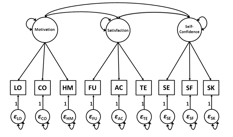
Figure 14.1: Factor model of the School Attitudes Questionnaire

The circles \(ε_{LO}\) through \(ε_{SK}\) at the bottom of Figure 14.1 are so-called residual factors. Just as with path analysis, residual factors in factor analysis are unobserved, latent factors that represent all factors that fall outside the model but may influence the states of the corresponding observed indicator variables. In the context of factor analysis, these residual factors can be considered ‘container variables’ that represent everything that is specific to the associated observed indicator variable (as opposed to everything that the observed indicator variables have in common, as represented by the common factors). The residual factors also reflect measurement error. The variance of a residual factor therefore partly consists of variance due to random error fluctuations (i.e., measurement error; unsystematic variance) and partly of specific variable variance (i.e., due to unmeasured causes; systematic variance). The directional effects from the residual factors to the corresponding observed indicator variables are accompanied by the scaling constant ‘1’ for reasons of identification (which is explained in more detail in section 14.4).

14.3 Symbolic explanation of a factor model

Figure 14.2 is again a graphical representation of the factor model of the SAQ, but now also includes the Greek symbols that are associated with the common factors (‘\(ξ\)’, or ‘ksi’) and the directional effects between the common factors and observed indicator variables (‘\(λ\)’, or ‘lambda’). Using these symbols, the relationships between the observed indicator variables and the underlying common factor as presented in Figure 2 can be given by the following equations:

\[\begin{align} \mathrm{x}_1 = \lambda_{11}\xi_1+\varepsilon_1, \tag{14.1} \\ \mathrm{x}_2 = \lambda_{21}\xi_1+\varepsilon_2, \tag{14.2} \\ \mathrm{x}_3 = \lambda_{31}\xi_1+\varepsilon_3, \tag{14.3} \\ \mathrm{x}_4 = \lambda_{42}\xi_2+\varepsilon_4, \tag{14.4} \\ \mathrm{x}_5 = \lambda_{52}\xi_2+\varepsilon_5, \tag{14.5} \\ \mathrm{x}_6 = \lambda_{62}\xi_2+\varepsilon_6, \tag{14.6} \\ \mathrm{x}_7 = \lambda_{73}\xi_3+\varepsilon_7, \tag{14.7} \\ \mathrm{x}_8 = \lambda_{83}\xi_3+\varepsilon_8, \tag{14.8} \\ \mathrm{x}_9 = \lambda_{93}\xi_3+\varepsilon_9, \tag{14.9} \end{align}\]

where \(\mathrm{x}_1\) through \(\mathrm{x}_9\) are the nine observed indicator variables, \(\xi_1\), \(\xi_2\) and \(\xi_3\) are the common factors Motivation, Satisfaction, and Self-Confidence respectively, and \(\varepsilon_1\) through \(\varepsilon_9\) are the residual factors of the associated \(\mathrm{x}_1\) through \(\mathrm{x}_9\). Parameters \(\lambda_{11}\) through \(\lambda_{93}\) are factor loadings. Using the equations, we can again see that each of the observed variables is only affected by one of the common factors. Note also that each of the observed variables is affected by its associated residual factor.

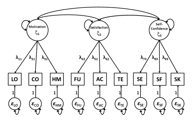
Figure 14.2: Factor Model of the School Attitudes Quetsionnaire

Instead of writing down the equation for each observed variable, the equations for the observed variables x1 through x9 can also be written in matrix form:

\[\begin{equation} \mathbf{x} = \mathbf\Lambda \mathbf\xi + \mathbf{\varepsilon}, \tag{14.10} \end{equation}\]

where \(\mathbf{x}\) is a vector of all observed variables, \(\mathbf\xi\) is a vector of all common factors, \(\mathbf\varepsilon\) is a vector of all residual factors, and \(\mathbf\Lambda\) is a matrix of factor loadings. \[ \mathbf{x}= \begin{bmatrix} x_1\\x_2\\x_3\\x_4\\x_5\\x_6\\x_7\\x_8\\x_9 \end{bmatrix}, \mathbf\xi = \begin{bmatrix} \xi_1\\\xi_2\\\xi_3 \end{bmatrix}, \mathbf\varepsilon = \begin{bmatrix} \varepsilon_1\\\varepsilon_2\\\varepsilon_3\\\varepsilon_4\\\varepsilon_5\\\varepsilon_6\\\varepsilon_7\\\varepsilon_8\\\varepsilon_9 \end{bmatrix}, \text{and } \mathbf\Lambda = \begin{bmatrix} \lambda_{11}&0&0\\\lambda_{21}&0&0\\\lambda_{31}&0&0\\0&\lambda_{42}&0\\0&\lambda_{52}&0\\0&\lambda_{62}&0\\0&0&\lambda_{73}\\0&0&\lambda_{83}\\0&0&\lambda_{93} \end{bmatrix}. \]

Matrix \(\mathbf\Lambda\) contains nine nonzero elements: \(\lambda_{11}\) through \(\lambda_{93}\). Like the regression slopes in the Beta matrix (\(\mathbf{B}\)), rows represent the outcomes (here, indicators) and columns represent the predictors (here, common factors). So the factor loading \(\lambda_{ij}\) represents the regression of variable \(i\) on common factor \(j\). When the factor model is specified such that variable \(i\) does not load on common factor \(j\), then that specific element \(\lambda_{ij}\) is fixed to zero. Specifically, the pattern of matrix \(\mathbf\Lambda\) specifies the measurement structure of the factor model. In our example, \(\mathbf\Lambda\) contains many elements that are fixed to zero because each indicator variable loads only on one of three common factors. Such a pattern of factor loadings is sometimes referred to as ‘simple structure’.

Substituting these matrices into Equation (14.10) gives:

\[\begin{equation} \begin{bmatrix} x_1\\x_2\\x_3\\x_4\\x_5\\x_6\\x_7\\x_8\\x_9 \end{bmatrix}=\begin{bmatrix} \lambda_{11} & 0 & 0 \\ \lambda_{21} & 0 & 0 \\ \lambda_{31} & 0 & 0 \\ 0 & \lambda_{42} & 0 \\ 0 & \lambda_{52} & 0 \\ 0 & \lambda_{62} & 0 \\ 0 & 0 & \lambda_{73} \\ 0 & 0 & \lambda_{83} \\ 0 & 0 & \lambda_{93} \end{bmatrix}\begin{bmatrix}\xi_1\\\xi_2\\\xi_3 \end{bmatrix}+\begin{bmatrix}\varepsilon_1\\\varepsilon_2\\\varepsilon_3\\\varepsilon_4\\\varepsilon_5\\\varepsilon_6\\\varepsilon_7\\\varepsilon_8\\\varepsilon_9 \end{bmatrix} \tag{14.11} \end{equation}\]

and evaluation gives:

\[\begin{equation} \begin{bmatrix} x_1\\x_2\\x_3\\x_4\\x_5\\x_6\\x_7\\x_8\\x_9 \end{bmatrix} = \begin{bmatrix} \lambda_{11}\xi_1+\varepsilon_1\\ \lambda_{21}\xi_1+\varepsilon_2\\ \lambda_{31}\xi_1+\varepsilon_3\\ \lambda_{42}\xi_2+\varepsilon_4\\ \lambda_{52}\xi_2+\varepsilon_5\\ \lambda_{62}\xi_2+\varepsilon_6\\ \lambda_{73}\xi_3+\varepsilon_7\\ \lambda_{83}\xi_3+\varepsilon_8\\ \lambda_{93}\xi_3+\varepsilon_9 \end{bmatrix}. \tag{14.12} \end{equation}\]

Here, we can see that the equations for variables \(\mathrm{x}_1\) through \(\mathrm{x}_9\) are the same as separate Equations (14.1) through (14.9).

We now have an expression for the scores on the observed indicator variables. However, in standard SEM we do not model the observed scores directly, but rather the variances and covariances of the observed scores. Therefore, we need to find an expression for the model-implied covariance matrix. Using Equation (14.10) and some covariance algebra, we obtain the expression for the variances and covariances of \(\mathbf{x}\), called \(\mathbf\Sigma_{\text{model}} = \text{COV}(\mathbf{x},\mathbf{x})\):

\[\begin{equation} \mathbf\Sigma_{\text{model}} = \mathbf\Lambda \mathbf\Phi \mathbf\Lambda^\text{T} + \mathbf\Theta, \tag{14.13} \end{equation}\]

where the variances and covariances of the common factors are represented by \(\text{COV}(\mathbf\xi,\mathbf\xi) = \mathbf\Phi\), and the variances and covariances of the residual factors represented by \(\text{COV}(\mathbf\varepsilon,\mathbf\varepsilon) = \mathbf\Theta\). The matrix \(\mathbf\Lambda\) contains the common factor loadings, and \(\mathbf\Lambda^\text{T}\) denotes the transpose of the matrix \(\mathbf\Lambda\). Derivations of Equation (14.13) are given in the Appendix at the end of this chapter.

Matrix \(\mathbf\Phi\) is a symmetric matrix and contains the variances and covariances of the common factors \(\mathbfξ\). For the model given in Equation (14.12), matrix \(\mathbf\Phi\) is:

\[\begin{equation} \mathbf\Phi = \begin{bmatrix} \phi_{11}\\\phi_{21}&\phi_{22}\\\phi_{31}&\phi_{32}&\phi_{33}\\ \end{bmatrix}, \tag{14.14} \end{equation}\]

where the diagonal elements \(φ_{11}\), \(φ_{22}\), \(φ_{33}\) represent the variances of common factors \(ξ_1\), \(ξ_2\), and \(ξ_3\), respectively, and the off-diagonal elements represent the covariances between the common factors, e.g., the element \(φ_{21}\) represents the covariance between common factors \(ξ_1\) and \(ξ_2\).

Matrix \(\mathbf\Theta\) is a symmetric matrix and contains the variances and covariances of the residual factors. It is often assumed that the residual factors do not covary with each other, so that matrix \(\mathbf\Theta\) is a diagonal matrix with residual variances only. However, in some applications covariances between (some) residual factors are allowed, which are then specified by nonzero off-diagonal elements of matrix \(\mathbf\Theta\). The \(\mathbf\Theta\) matrix for our illustrative example from the Figure 14.2 model is:

\[\begin{equation} \mathbf\Theta = \begin{bmatrix} \theta_{11}\\ 0&\theta_{22}\\ 0&0&\theta_{33}\\ 0&0&0&\theta_{44}\\ 0&0&0&0&\theta_{55}\\ 0&0&0&0&0&\theta_{66}\\ 0&0&0&0&0&0&\theta_{77}\\ 0&0&0&0&0&0&0&\theta_{88}\\ 0&0&0&0&0&0&0&0&\theta_{99} \end{bmatrix}, \tag{14.15} \end{equation}\]

where \(θ_{11}\) through \(θ_{99}\) represent the variances of the residual factors of \(\mathrm{x}_1\) through \(\mathrm{x}_9\). These residual variances represent the variance of the associated indicator variable that is not represented by the underlying common factors. They can be interpreted as variance that is unexplained by the model.

In Figure 3, the \(\mathbf\Phi\) and \(\mathbf\Theta\) parameters representing common factor variances and covariances and residual factor variances and covariances are added to the graphical display.

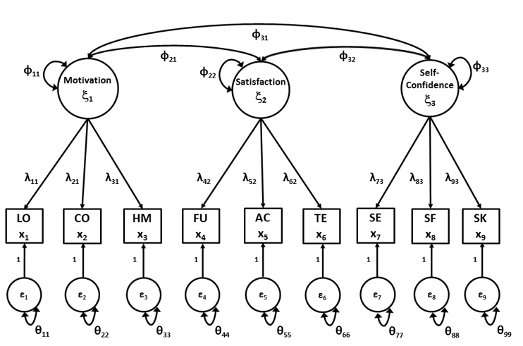
Figure 14.3: Factor model of the School Attitudes Questionnaire including common factor and residual factor (co)variance parameters

Now that we have found the general expression for the variances and covariances as a function of model parameters of a factor model, we can evaluate Equation (14.13) of our illustrative example. Substitution of the \(\mathbf\Lambda\), \(\mathbf\Phi\), and \(\mathbf\Theta\) of our example yields:

\(\mathbf\Sigma_{\text{model}} = \mathbf\Lambda \mathbf\Phi \mathbf\Lambda^\text{T} + \mathbf\Theta\), where:

\[ \mathbf\Lambda \mathbf\Phi \mathbf\Lambda^\text{T} = \begin{bmatrix} \lambda_{11}&0&0\\\lambda_{21}&0&0\\\lambda_{31}&0&0\\0&\lambda_{42}&0\\0&\lambda_{52}&0\\0&\lambda_{62}&0\\0&0&\lambda_{73}\\0&0&\lambda_{83}\\0&0&\lambda_{93} \end{bmatrix} \begin{bmatrix} \phi_{11}\\\phi_{21}&\phi_{22}\\\phi_{31}&\phi_{32}&\phi_{33} \end{bmatrix} \begin{bmatrix} \lambda_{11}&\lambda_{21}&\lambda_{31}&0&0&0&0&0&0\\0&0&0&\lambda_{42}&\lambda_{52}&\lambda_{62}&0&0&0\\0&0&0&0&0&0&\lambda_{73}&\lambda_{83}&\lambda_{93} \end{bmatrix} \]

and thus \(\mathbf\Sigma_{\text{model}}\) is given by:

\[\begin{equation} \mathbf\Sigma_{\text{model}} = \begin{bmatrix} \lambda^2_{11} \varphi_{11} +\theta_{11} \\ \lambda_{11}\lambda_{21}\varphi_{11} & \lambda^2_{21}\varphi_{11}+\theta_{22} \\ \lambda_{11}\lambda_{31}\varphi_{11} & \lambda_{21}\lambda_{31}\varphi_{11} & \lambda^2_{31}\varphi_{11}+\theta_{33}\\ \lambda_{11}\lambda_{42} \varphi_{21} & \lambda_{21}\lambda_{42}\varphi_{21} & \lambda_{31}\lambda_{42}\varphi_{21} & \lambda^2_{42}\varphi_{22}+\theta_{44}\\ \lambda_{11}\lambda_{52} \varphi_{21} & \lambda_{21}\lambda_{52} \varphi_{21} & \lambda_{31}\lambda_{52}\varphi_{21} & \lambda_{42}\lambda_{52}\varphi_{22} & \lambda^2_{52}\varphi_{22}+\theta_{55}\\ \lambda_{11}\lambda_{62}\varphi_{21} & \lambda_{21}\lambda_{62} \varphi_{21} & \lambda_{31}\lambda_{62}\varphi_{21} & \lambda_{42}\lambda_{62}\varphi_{22} & \lambda_{52}\lambda_{62}\varphi_{22} & \lambda^2_{62}\varphi_{22}+\theta_{66}\\ \lambda_{11}\lambda_{73}\varphi_{31} & \lambda_{21}\lambda_{73}\varphi_{31} & \lambda_{31}\lambda_{73}\varphi_{31} & \lambda_{42}\lambda_{73}\varphi_{32} & \lambda_{52}\lambda_{73}\varphi_{32} &\lambda_{62}\lambda_{73}\varphi_{32} & \lambda^2_{73} \varphi_{33}+\theta_{77}\\ \lambda_{11}\lambda_{83} \varphi_{31} & \lambda_{21}\lambda_{83}\varphi_{31} &\lambda_{31}\lambda_{83}\varphi_{31} & \lambda_{42}\lambda_{83}\varphi_{32} & \lambda_{52}\lambda_{83}\varphi_{32} & \lambda_{62}\lambda_{83}\varphi_{32} & \lambda_{72}\lambda_{83}\varphi_{32} & \lambda^2_{83}\varphi_{33}+\theta_{88}\\ \lambda_{11}\lambda_{93} \varphi_{31} & \lambda_{21}\lambda_{93} \varphi_{31} & \lambda_{31}\lambda_{93}\varphi_{31} & \lambda_{42}\lambda_{93}\varphi_{32} & \lambda_{52}\lambda_{93}\varphi_{32} & \lambda_{62}\lambda_{93}\varphi_{32} & \lambda_{73}\lambda_{93}\varphi_{32} & \lambda_{83}\lambda_{93}\varphi_{32} & \lambda^2_{93}\varphi_{33}+\theta_{99} \end{bmatrix} \tag{14.16} \end{equation}\]

We can thus evaluate whether the factor model gives a good description of the linear dependencies between the observed variables by evaluating \(\mathbf\Sigma_{population} = \mathbf\Sigma_{model}\), where \(\mathbf\Sigma_{population}\) is given by:

\[\begin{equation} \mathbf\Sigma_{population}= \begin{bmatrix} \sigma_{11} \\ \sigma_{21} & \sigma_{22} \\ \sigma_{31} & \sigma_{32} & \sigma_{33} \\ \sigma_{41} & \sigma_{42} & \sigma_{43} & \sigma_{44} \\ \sigma_{51} & \sigma_{52} & \sigma_{53} & \sigma_{54} & \sigma_{55} \\ \sigma_{61} & \sigma_{62} & \sigma_{63} & \sigma_{64} & \sigma_{65} & \sigma_{66} \\ \sigma_{71} & \sigma_{72} & \sigma_{73} & \sigma_{74} & \sigma_{75} & \sigma_{76} & \sigma_{77} \\ \sigma_{81} & \sigma_{82} & \sigma_{83} & \sigma_{84} & \sigma_{85} & \sigma_{86} & \sigma_{87} & \sigma_{88} \\ \sigma_{91} & \sigma_{92} & \sigma_{93} & \sigma_{94} & \sigma_{95} & \sigma_{96} & \sigma_{97} & \sigma_{98} & \sigma_{99} \end{bmatrix}. \tag{14.17} \end{equation}\]

14.4 Identification of model parameters in a factor model

The population variances (\(\sigma_{ii}\)), and covariances (\(\sigma_{ij}\)) that feature in Equation (14.17) can be estimated with sample variances (\(s_{ii}\)), and covariances (\(s_{ij}\)). Similar to the identification of path models, the factor model is identified if it is possible to uniquely express each of the model parameters that feature in Equation (14.16) as functions of the variances and covariances of Equation (14.17). However, the identification of latent factors requires additional restrictions. Because latent factors are unobserved variables, we do not know the scales of measurements of these variables. Because the scales of the common factors are not defined, it is not possible to estimate both the variance and factor loading of a latent factor. To give scales to the latent factors, one can either fix the factor variance or one of the factor loadings at a nonzero value. The identification of residual factors—which also appear in path models—is usually done by using a scaling constant ‘1’ for the associated residual factor loading (i.e., the direct effect of the residual factor on the associated observed variable). These restrictions are applied by default by most computer programs.

For the identification of common factors, the researcher can chose between the two types of identification restrictions: through restriction of common-factor variances or through restriction of factor loadings. For example, to identify the common factors from our illustrative example, one can fix either the factor variances at a nonzero value (e.g., \(\varphi_{11} = 1, \varphi_{22} = 1, \varphi_{33} = 1\)) or one factor loading for each factor (e.g., \(\lambda_{11} = 1, \lambda_{22} = 1\), and \(\lambda_{33} = 1\). As the scaling constant is usually ‘1’, these two types of identification constraints are referred to as: the ‘unit variance identification constraint’ (UVI constraint) and the ‘unit loading identification constraint’ (ULI constraint). The UVI method is also referred to as the ‘fixed-factor’ method, and the ULI method is referred to as the ‘marker-variable’ or ‘reference-variable’ method. A third method is related to ULI, but instead of constraining a single loading to 1, all loadings are estimated under the constraint that the mean of the loadings is 1—this is called the ‘effects-coding’ method.

Traditionally, we would choose a “marker” or “reference” variable that is thought to best represent the latent construct (i.e., the perfect indicator, if it did not have measurement error), and we would fix the loading of that indicator to 1 (ULI constraint). The logic behind ULI was that fixing the factor loading to 1 implied a 1-unit increase in the reference indicator (on average) for each 1-unit increase in the common factor. Thus, the common factor was often said to “be on the same scale” as the reference indicator. However, that would only be true if the reference indicator had no measurement error (implying its residual variance could be fixed to zero). Holding the reliability of an indicator (i.e., the proportion of its variance that is common-factor variance ) constant, the more measurement error the indicator has, the greater its estimated residual variance and the lower its estimated factor loading would be. So when the reference indicator does have measurement error (which we assume implicitly, otherwise we wouldn’t need a common-factor model for the latent construct), the ULI method sets the scale of the common factor to the scale of the common-factor component of the reference indicator, not to its total (i.e., its observed) scale (Steiger, 2002).

So although the ULI method has been most popular in SEM for decades, its popularity is based on a misconception. Latent variables have no implicit scale because they are unobserved by definition, and no statistical trick can give them a meaningful scale. Units of standard deviation are familiar because we often use standardized effect sizes in other contexts (e.g., Cohen’s d is a standardized mean difference, a correlation is a standardized simple regression slope). Standardized estimates are available regardless of the scaling constraint, so the UVI / fixed-factor method is not necessarily any better—both methods lead to identical model fit, and the estimated factor loadings are proportionally equivalent relative to the factor variance, whether it is fixed to 1 or set using the common-factor component of an indicator. However, the \(SE\)s of the factor loadings are sensitive to the different identification methods (Gonzalez & Griffin, 2001), so Wald \(z\) tests of significance for factor loadings are affected. This may only lead to different conclusions about the null hypothesis that \(λ_{ij} = 0\) when indicators have much more measurement error than common-factor variance, or when \(N\) is quite low. However, it is troubling to think that an estimated \(SE\) depends on an arbitrary scaling constraint. The UVI / fixed-factor method may be preferable if only because the specified factor variance is arbitrary anyway, and ULI seems to imply that one of the factor loadings is a known quantity.

The effects-coding method of identification has the benefit of estimating the factor variance without specifying a single variable as the ideal reference indicator. Instead of fixing one loading to 1, it estimates all loadings under the constraint that the average loading (per construct) is 1, or equivalently, that the factor loadings sum to the number of indicators (\(N_i\)). This is equivalent to constraining one loading to be \(N_i\) minus the remaining factor loadings. Thus, the indicator with the “average” amount of common-factor variance would have a factor loading of 1, and loadings above 1 belong to the indicators that have more common-factor variance than average (among the indicators used in the analysis).

Although effects coding was originally conceived as a “non-arbitrary” method of scaling the latent construct (Little, Slegers, & Card, 2006), that was based on the same misconception as believing the ULI sets the latent construct’s scale identical to the reference indicator’s scale. However, the effects-coding method is advantageous in scenarios when fixing the latent variance is suboptimal. For example, we can only scale the residual variance of an endogenous common factor, rather than the total variance, and fixing a residual variance to 1 may be intuitively unappealing (although it is as arbitrary as fixing the total variance).

When a factor has fewer than three indicators, these scaling methods are not sufficient for identification. We devote a later chapter to single-indicator constructs, which can be used to model the effects of observed variables (e.g., sex or age) on latent common factors¹⁸. However, constructs with only two indicators have a complicated status. With only two indicators, there are three observed pieces of information: two variances and a single covariance, which represents the shared (common) variance between the indicators. That is not enough to identify the five pieces of information we could estimate (two residual variances, one factor variance, and two factor loadings), so we need to fix two pieces of information instead of just one. Using the ULI orientation is intuitively appealing in this situation, because when you fix both factor loadings to 1, the estimated common-factor variance is the observed covariance (i.e., the observed common variance). The UVI orientation would be to fix the factor variance to 1, but we still need another constraint for just-identification, which we can achieve by constraining the estimated factor loadings to equality (i.e., estimate one loading, but set both the loadings to that one value). Effects coding is not possible with only two indicators.

To make the situation more complicated, you can estimate a two-indicator factor with only one constraint, but only when the factor has a nonzero covariance with another factor in the model. The covariances of the two indicators with other indicators in the other factor will be enough to empirically identify the factor loading(s) and/or factor variance of the two-indicator factor—but only if the factor covariance is substantial. If the factor covariance is close to zero, the model will still be empirically underidentified. It is therefore preferable to ensure identification, ideally by fixing both factor loadings to 1 so that the freely estimated factor variance represents what it literally is: the covariance between the indicators.

14.5 Fitting a factor model using lavaan

The lavaan script for fitting a factor model resembles the script for fitting a path model. We again use equations to specify the model, but we now use the “=~” operator to define the common factors. Whereas the “~” operator specifies regression paths that point from predictor(s) on the right-hand side to outcome(s) on the left-hand side, the “=~” operator specifies regression paths (called factor loadings) that point from the predictor (common factor) on the left-hand side to the outcomes (indicators) on the right-hand side. Script 14.1 fits the three-factor model from Figure 14.3 to the covariance matrix from observed scores of the SAQ that was administered to 915 school pupils.

Script 14.1

## observed covariance matrix
obsnames <- c("learning","concentration","homework","fun",
            "acceptance","teacher","selfexpr","selfeff","socialskill")
values <- c(30.6301,
            26.9452, 56.8918,
            24.1473, 31.6878, 53.2488,
            16.3770, 18.4153, 16.8599, 27.9758,
             7.8174,  9.6851, 12.0114, 12.8765, 47.0970,
            13.6902, 16.9232, 12.9326, 17.2880, 12.3672, 29.0119,
            15.3122, 24.2849, 21.4935, 12.9621, 13.9909, 11.6333, 59.5343,
            13.4457, 21.8158, 18.8545,  7.3931, 12.2333,  7.1434, 29.7953, 49.2213,
             6.6074, 12.7343, 12.5768,  6.4065, 13.4258,  6.1429, 26.0849, 23.6253, 40.0922)

saqcov <- getCov(values, names = obsnames)

## specify model
saqmodel <- '
    # define latent common factors
    Motivation =~ L11*learning + L21*concentration + L31*homework
    Satisfaction =~ L42*fun + L52*acceptance + L62*teacher
    SelfConfidence =~ L73*selfexpr + L83*selfeff + L93*socialskill

    # indicator residual variances (or use "auto.var = TRUE") 
    learning ~~ TH11*learning
    concentration ~~ TH22*concentration
    homework ~~ TH33*homework
    fun ~~ TH44*fun
    acceptance ~~ TH55*acceptance
    teacher ~~ TH66*teacher
    selfexpr ~~ TH77*selfexpr
    selfeff ~~ TH88*selfeff
    socialskill ~~ TH99*socialskill

    # common factor variances (or use "auto.var = TRUE")
      Motivation ~~ F11*Motivation
      Satisfaction ~~ F22*Satisfaction
      SelfConfidence ~~ F33*SelfConfidence
    # factor covariances (or use "auto.cov.lv.x = TRUE")
    Motivation ~~ F21*Satisfaction
    Motivation ~~ F31*SelfConfidence
    Satisfaction ~~ F32*SelfConfidence

    # OPTIONAL: manually specify scaling constraints
    # UVI / fixed-factor method (or use "std.lv = TRUE")
        # F11 == 1
        # F22 == 1
        # F33 == 1
    # ULI / marker-variable / reference-variable method
      # (or use "auto.fix.first = TRUE")
        # L11 == 1
        # L42 == 1
        # L73 == 1
    # effects-coding method (MUST specify in syntax)
      # NOTE: 3 different ways yield the same solution
    (L11 + L21 + L31) / 3 == 1 # mean(Lambda) = 1
    L42 + L52 + L62 == 3       # sum(Lambda) = number of indicators
    L73 == 3 – L83 – L93       # 1 lambda = difference between the sum and remaining loadings
    '
## fit model
saqmodelOut <- lavaan(saqmodel, sample.cov = saqcov, 
                      sample.nobs = 915, likelihood = "wishart")
## results
summary(saqmodelOut, fit = TRUE, standardized = TRUE, rsquare = TRUE)
## parameter matrices
lavInspect(saqmodelOut, "est")

The first part of the script, where the observed covariance matrix is created, is not different from when fitting a path model. Differences are present in the model specification, where we need to define the common factors and additional parameters that are specific to the factor model.

First, we define common factors by specify their factor loadings (\(λ_{ij}\), the regression paths pointing from a common factor to an observed indicator in Figure 14.3.

saqmodel <- '
    # define latent common factors
    Motivation =~ L11*learning + L21*concentration + L31*homework
    Satisfaction =~ L42*fun + L52*acceptance + L62*teacher
    SelfConfidence =~ L73*selfexpr + L83*selfeff + L93*socialskill

The operator (“=~”) defines the common factor, where the name on the left-hand side of the operator is the common factor. As far as the software is concerned, it is only an arbitrary label, so you can choose any name you want, but it should not be a variable name that exists in the input data. The names on the right-hand side of the operator are the observed variables that are its reflective indicators, and whose names must appear in the input data. Note that (just as with the path model) the residual error term is not explicitly included in the formula. These equations therefore refer to the pattern of factor loadings (\(\mathbfΛ\)).

We use labels for the estimates of the factor loadings, where the label refers to the position of the regression coefficient in the \(\mathbfΛ\) matrix. For example, the factor loadings of the observed indicators of Motivation are positioned in the first column, rows one, two and three, and therefore we use the labels “L11”, “L21”, and “L31”:

Motivation =~ L11*learning + L21*concentration + L31*homework

The residual errors are specified in the same way as they are with the path model, using the double tildes (~~) to represent two-headed arrows. These are the residual terms that are represented in the theta matrix (\(\mathbfΘ\)). As there are no covariances between residual factors specified in our model, this matrix is diagonal. That is, the diagonal elements of the symmetric \(\mathbfΘ\) are the indicators’ residual variances, and all residual covariances are fixed to zero. We use labels “TH11” through “TH99” to represent the 1st-row/1st-column element through the 9th-row/9th-column element.

    # indicator residual variances (or use "auto.var = TRUE") 
    learning ~~ TH11*learning
    concentration ~~ TH22*concentration
    homework ~~ TH33*homework
    fun ~~ TH44*fun
    acceptance ~~ TH55*acceptance
    teacher ~~ TH66*teacher
    selfexpr ~~ TH77*selfexpr
    selfeff ~~ TH88*selfeff
    socialskill ~~ TH99*socialskill

Note, however, that this syntax can be left out if you use an additional lavaan argument to automatically (auto.) estimate the variance (var):

saqmodelOut <- lavaan(saqmodel, sample.cov = saqcov, 
                      sample.nobs = 915, likelihood = "wishart",
                      auto.var = TRUE)

Next, we need to specify the variances and covariances between the common factors (\(\mathbfΦ\))¹⁹. We use labels “F11” to “F33” for the variances, and the covariances are labeled with “F21”, “F31” and “F32”.

    # common factor variances (or use "auto.var = TRUE")
      Motivation ~~ F11*Motivation
      Satisfaction ~~ F22*Satisfaction
      SelfConfidence ~~ F33*SelfConfidence
    # factor covariances (or use "auto.cov.lv.x = TRUE")
    Motivation ~~ F21*Satisfaction
    Motivation ~~ F31*SelfConfidence
    Satisfaction ~~ F32*SelfConfidence

Similar to residual variances, common-factor variances can be omitted from the model syntax if you use the argument “auto.var = TRUE”. Likewise, you can omit common-factor covariances from the model syntax if you use the argument “auto.cov.lv.x = TRUE”.

Now we have specified all parameters of our factor model that are free to be estimated. However, although our model has positive degrees of freedom, it is still not identified. We must fix either the factor variances at a nonzero value or constrain at least one factor loading for each factor to give the factors a scale. Script 14.1 shows three ways to specify within the model syntax the scaling constraints necessary to identify the model. First we demonstrate the UVI (fixed-factor) constraint:

    # UVI / fixed-factor method (or use "std.lv = TRUE")
    F11 == 1
    F22 == 1
    F33 == 1

Note that the “==” operator (translated: “is equal to”) can only have constants on the left- and right-hand sides. These can be explicit constants (e.g., “1”) or parameter labels (e.g., “F11”), but variables can never be part of an equality constraint²⁰. Also note that you are not required to specify this constraint explicitly in the model syntax. Instead, you can tell lavaan to standardize (std.) each latent variable (lv):

saqmodelOut <- lavaan(saqmodel, sample.cov = saqcov, 
                      sample.nobs = 915, likelihood = "wishart",
                      std.lv = TRUE)

The alternative method to give scales to the common factors would be to fix one of the factor loadings of each common factor. Because software is ignorant of which variable might be preferred as a reference indicator, the default is typically to use the “first” indicator per factor as a reference indicator; however, if no indicator stands out as the ideal indicator, then there is little justification for use the ULI constraint. The ULI method can be specified explicitly in the model syntax:

    # ULI / marker-variable / reference variable method
      # (or use "auto.fix.first = TRUE")
        # L11 == 1
        # L42 == 1
        # L73 == 1

Or, as noted in the syntax comment, you can omit constraints from the syntax by telling lavaan you want to automatically (auto.) fix the first loading to 1:

saqmodelOut <- lavaan(saqmodel, sample.cov = saqcov, 
                      sample.nobs = 915, likelihood = "wishart",
                      auto.fix.first = TRUE)

When there is not an ideal indicator to use as the reference variable, but the research wants to estimate factor variances, the effects-coding method can be used.

    # effects-coding method (MUST specify in syntax)
      # NOTE: 3 different ways yield the same solution
    (L11 + L21 + L31) / 3 == 1 # mean(Λ) = 1
    L42 + L52 + L62 == 3       # sum(Λ) = number of indicators
    L73 == 3 – L83 – L93       # 1 λ = difference between the
                                 # sum and remaining loadings

Note the three equivalent ways of specifying the necessary constraint, each of which is demonstrated using a different factor’s indicators. Note also that effects coding does not have an argument in lavaan, so it must be specified in model syntax using parameter labels (which would not be required when using the auto.fix.first or std.lv arguments).

Finally, we run the model with the lavaan function. The arguments are the model syntax (saqmodel), the covariance matrix as input data (saqcov), and the sample size (\(N = 915\)). We still use Wishart likelihood when we fit our model only to the sample covariance matrix, but unlike with path models, we no longer need to set the argument fixed.x = FALSE because all observed variables are endogenous .

## run model
saqmodelOut <- lavaan(saqmodel, sample.cov = saqcov, 
                      sample.nobs = 915, likelihood = "wishart")

There is a dedicated “wrapper” function (i.e., a function that calls lavaan() with specific defaults turned on) called cfa(). Specifically, cfa() calls lavaan() with the arguments auto.fix.first, auto.var, and auto.cov.lv.x set to TRUE. To use UVI instead of ULI, you can implicitly set auto.fix.first back to FALSE by setting std.lv = TRUE. Effects coding, however, requires calling lavaan() directly. Script 14.2 yields the same results as Script 14.1 (specifically, using the UVI constraint) but with many fewer lines of syntax. ### Script 14.2 {-}

## observed covariance matrix
obsnames <- c("learning","concentration","homework","fun",
            "acceptance","teacher","selfexpr","selfeff","socialskill")
values <- c(30.6301,
            26.9452, 56.8918,
            24.1473, 31.6878, 53.2488,
            16.3770, 18.4153, 16.8599, 27.9758,
             7.8174,  9.6851, 12.0114, 12.8765, 47.0970,
            13.6902, 16.9232, 12.9326, 17.2880, 12.3672, 29.0119,
            15.3122, 24.2849, 21.4935, 12.9621, 13.9909, 11.6333, 59.5343,
            13.4457, 21.8158, 18.8545,  7.3931, 12.2333,  7.1434, 29.7953, 49.2213,
             6.6074, 12.7343, 12.5768,  6.4065, 13.4258,  6.1429, 26.0849, 23.6253, 40.0922)

saqcov <- getCov(values, names = obsnames)

## specify model
saqmodel <- '# define latent common factors
    Motivation =~ learning + concentration + homework
    Satisfaction =~ fun + acceptance + teacher
    SelfConfidence =~ selfexpr + selfeff + socialskill
    '
## run model
saqmodelOut <- cfa(saqmodel, sample.cov = saqcov, sample.nobs = 915,
                   std.lv = TRUE, likelihood = "wishart")
## output
summary(saqmodelOut, fit = TRUE, standardized = TRUE, rsquare = TRUE)
## parameter matrices
lavInspect(saqmodelOut, "est")

We request results of the analysis along with the standardized solution, model fit measures, and R2 for the indicators (i.e., proportion of variance explained by factors):

## output
summary(saqmodelOut, standardized = TRUE, fit = TRUE, rsquare = TRUE)

The lavaan summary() output is split into several parts, with information about model fit appearing first (which can also be found in the fitMeasures() output). The remaining sections can all be found in the parameterEstimates() output. “Latent Variables” contains the results of the regression equations (i.e., factor loadings), “Covariances” contains the parameter estimates of the common-factor covariances, and “Variances” contains the variances of the common factors and residual variances of the observed indicators. The bottom section contains the estimated \(R^2\) for each endogenous variable (i.e., indicators). The standardized solution is discussed in more detail in the following chapter.

To obtain the parameter estimates in matrix format (\(\mathbfΛ\), \(\mathbfΦ\), and \(\mathbfΘ\)), use the lavInspect() function. Note, however, that lavaan refers to \(\mathbfΦ\) as \(\mathbfΨ\) (“Psi”).

lavInspect(saqmodelOut, "est")

When we introduced path model notation in Chapter 3, we used Psi to represent the matrix of exogenous (co)variances and endogenous residual (co)variances. After we introduce the full SEM, which combines a path model with a factor model, lavaan’s use of \(\mathbfΨ\) instead of \(\mathbfΦ\) will make more sense. For now, think of them as arbitrary labels—either way, we are talking about the covariance matrix of latent variables. The use of Φ implies the latent variables are exogenous, and the use of Ψ implies at least one latent variable may be endogenous, but the formulas work the same either way.

References

Gonzalez, R., & Griffin, D. (2001). Testing parameters in structural equation modeling: Every “one” matters. Psychological Methods, 6(3), 258–269. doi:10.1037//1082-989X.6.3.258

Little, T. D., Slegers, D. W., & Card, N. A. (2006). A non-arbitrary method of identifying and scaling latent variables in SEM and MACS models. Structural Equation Modeling, 13(1), 59–72. doi:10.1207/s15328007sem1301_3

Smits, J. A., & Vorst, H. C. M. (1982). Schoolvragenlijst voor basisonderwijs en voortgezet onderwijs (SVL). Handleiding voor gebruikers. Nijmegen: Berkhout Nijmegen.

Steiger, J. H. (2002). When constraints interact: A caution about reference variables, identification constraints, and scale dependencies in structural equation modeling. Psychological Methods, 7(2), 210–227. doi:10.1037//1082-989X.7.2.210

Appendix

Derivations of Equation 14.13

\[ \mathbf\Sigma = \text{COV}(\mathbf{x},\mathbf{x}) \Leftrightarrow \] (substitute Equation (14.13)

\[ \mathbf\Sigma = \text{COV}(\mathbf\Lambda \mathbf\xi + \mathbf\varepsilon, \mathbf\Lambda \mathbf\xi + \mathbf\varepsilon) \Leftrightarrow \]

(decompose)

\[ \mathbf\Sigma = \text{COV}(\mathbf\Lambda \mathbf\xi,\mathbf\Lambda \mathbf\xi) + \text{COV}(\mathbf\Lambda \mathbf\xi,\mathbf\varepsilon)+ \text{COV}(\mathbf\varepsilon,\mathbf\Lambda \mathbf\xi)+ \text{COV}(\mathbf\varepsilon,\mathbf\varepsilon) \Leftrightarrow \]

(residual factors are assumed not to covary with the common factors, \(COV(\mathbf\xi,\mathbf\varepsilon) = 0.\))

\[ \mathbf\Sigma = \text{COV}(\mathbf\Lambda \mathbf\xi,\mathbf\Lambda \mathbf\xi) + 0 + 0 + \text{COV}(\mathbf\varepsilon,\mathbf\varepsilon) \Leftrightarrow \] (place constants outside brackets).

\[ \mathbf\Sigma = \mathbf\Lambda \text{COV}(\mathbf\xi,\mathbf\xi)\mathbf\Lambda^{\text{T}} +\text{COV}(\mathbf\varepsilon,\mathbf\varepsilon)\Leftrightarrow \]

(variances and covariances of \(\mathbf\xi\) and \(\mathbf\varepsilon\) are denoted \(\mathbf\Phi\) and \(\mathbf\Theta\))

\[ \mathbf\Sigma = \mathbf\Lambda \mathbf\Phi \mathbf\Lambda^\text{T} + \mathbf\Theta \]

---

18. This is necessary because the SEM matrices of regression coefficients only allow for effects of latent factors on observed variables (Λ) or of latent variables on latent variables (B). In path models, we actually treat all observed variables as single-indicator constructs, allowing us to use B.↩︎

19. The Greek letter “Phi” can be pronounced like “fee” (typical in U.S. English) or like it rhymes with “eye” (typical in U.K. English). The Greeks pronounce \(Φ\) as “fee,” but they also pronounce \(χ\) as “key” and \(π\) as “pee.” Unless you are actually speaking Greek, you are not required to conform to these conventions. By analogy, English, Germans, French, and Dutch (among others) all have very different pronunciations for the same letters of the alphabet (for example, E, I, H, J, R, V, W, U, and Z can differ quite a lot from language to language).↩︎

20. Functions of parameters can also be specified (e.g., “F11 == log(F22)” or “sqrt(L11) == abs(L42)”). Inequality constraints can also be specified, which will not fix a parameter but will constrain the range of values it could be. This is most commonly used to constrain variances to be positive (e.g., “F11 > 0”); however, such constrained estimation is not preferred because it can have unintended consequences (e.g., hides model misspecification, forces other parameter estimates to be biased, the model fit statistic is no longer distributed as a simple \(χ^2\) random variable under \(\text{H}_0\)).↩︎