28 Analysis of categorical outcomes

Until now we have focused on the analysis of continuous outcomes (endogenous variables in path models, indicators in factor models), and we have used the maximum likelihood (ML) estimator that assumes that the distribution of the scores on the observed variables are multivariate normal. Various robust estimators can be used when the assumption of multivariate normality cannot be met, which adjust the $χ^2$ test statistic and $SE$s for nonnormality, but those robust estimators still assume the data are continuous. When we want to analyse categorical data, adjusting for nonnormality is not sufficient because the parameters are not interpretable if the model does not take into account the categorical nature of the observed variables it is trying to explain.

The chapters on multiple groups and single-indicator constructs introduced how to incorporate categorical predictors into a SEM. In this chapter we will focus on how we can analyse categorical outcomes. When we have categorical data instead of continuous data, the responses are limited to a small number of values (e.g., 2, 3, or 4 response categories). To be able to analyse these responses, we assume that the categorical responses are representations of a continuous underlying variable, often called a “latent response” variable (distinct from a latent common factor). A latent response is a variable we would like to have measured (e.g., how happy you are) using a more sensitive instrument, but in practice we were only capable of measuring whether someone is in a particular range (e.g., whether they feel happy never, rarely, often, or always). The idea is that people with lower scores on the latent response are likely to indicate lower categories of the observed categorical response, whereas people with higher scores on the latent response are likely to indicate higher categories of the observed categorical response. We can think of each latent response as being a single-indicator construct, where the single indicator is the observed categorical response.

Figure 28.1 shows the relation between the underlying continuous variable ($\mathrm{y}^{*}$) and the observed categorical response ($\mathrm{y}$) for a dichotomous variable. Let’s consider this to be a test question, which is a common situation with binary indicators. In this example, the latent response variable $\mathrm{y}^{*}$ could be labelled “how well [they] understand this test question” or their “propensity for solving this problem”, and the observed binary response would simply be correct (1) or incorrect (0). Here, the difference between the answer “0” and “1” is determined by the threshold ($δ_1$), which represents “how well [they] need to understand this test question in order to get it correct”. When an individual’s unobserved $\mathrm{y}^{*}$ is below the threshold, we assume that the observed categorical response would be “0” (i.e., they do not understand well enough to get the question correct), whereas a latent response above the threshold would result in an observed response of “1” (i.e., they do understand well enough to get the question correct). When we assume this underlying variable follows a standard normal distribution (i.e., with $μ = 0$ and $σ = 1$), then the position of the threshold is the value of the standard normal distribution ($z$ score) that makes the area under the curve lower than (to the left of) the threshold equal to the proportion of observed responses of ‘0’ (i.e., what percentage got the question incorrect).

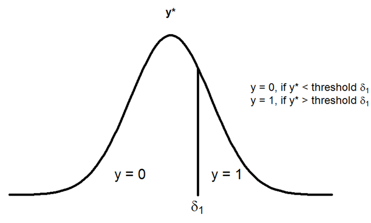
$A dichotomous response ($y$) and associated theshold ($δ_1$) for an underlying continuous variable $y^{*}$$

Figure 28.1: A dichotomous response ($y$) and associated theshold ($δ_1$) for an underlying continuous variable $y^{*}$

The information above applies to the situation when we have two response categories (dichotomous/binary data), but can easily be extended to multiple ordered response categories (polytomous/ordinal data). Additional thresholds define the classification of the observed categorical responses, where the number of thresholds ($c$) is equal the number of categories ($C$) minus one ($c = C − 1$). An example of a variable with three response categories is given in Figure 28.2.

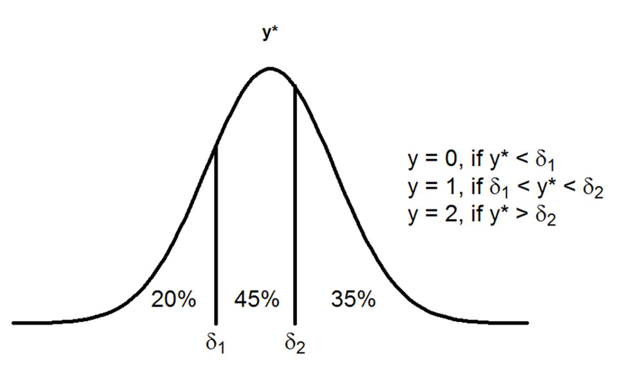
$The estimation of thresholds ($δ_1$ and $δ_2$): Observed categorical responses y are representations of underlying continuous scores $y^*$. There are 20%, 45%, and 35% observed responses in categories 0, 1, and 2 respectively. Cumulatively this is 20%, 65% (20 + 45), and 100% (20 + 45 + 35) of the entire distribution. The first threshold is located where the area under the curve to the left of the threshold is 20% ($δ_1 = Z_{20} = −0.842$). The second threshold is located where the area under the curve to the left of the threshold is 65% ($δ_2 = Z_{65} = 0.385$).$

Figure 28.2: The estimation of thresholds ($δ_1$ and $δ_2$): Observed categorical responses y are representations of underlying continuous scores $y^*$. There are 20%, 45%, and 35% observed responses in categories 0, 1, and 2 respectively. Cumulatively this is 20%, 65% (20 + 45), and 100% (20 + 45 + 35) of the entire distribution. The first threshold is located where the area under the curve to the left of the threshold is 20% ($δ_1 = Z_{20} = −0.842$). The second threshold is located where the area under the curve to the left of the threshold is 65% ($δ_2 = Z_{65} = 0.385$).

With multiple ordinal variables, we can estimate the correlations between their associated latent responses (called “polychoric” correlations) by relying on the assumption that the latent response variables are normally distributed. A polychoric correlation approximates what the Pearson correlation would be if the variables had been measured using a continuous scale that represented their true distributional form. In the special case that both observed categorical responses are binary, this estimate is called a “tetrachoric” correlation, but we can use the more general term polychoric correlation matrix to refer to these summary statistics.

When we fit a SEM to categorical outcomes, we therefore need to estimate thresholds, followed by the polychoric correlation matrix. Because the latent responses have not been observed, we fix $μ = 0$ and $σ = 1$ for identification, just like we do for latent common factors. Alternative estimators and adjustments to the $χ^2$ test statistic and $SE$s should be used to arrive at correct parameter estimates and model fit.

In the current chapter we will explain how to fit CFA models to categorical outcomes in lavaan using the diagonally weighted least squares (DWLS) estimator of parameters, which does not rely on assuming that data are normally distributed, or even continuous (although they certainly can be). Because the standard $χ^2$ test statistic and $SE$s have inflated Type I error rates, lavaan also provides a robust $χ^2$ and $SE$s. Models must be fitted to complete raw data rather than summary statistics. We will give two examples: one for binary item responses and one for three-category ordinal item responses. Because CFA models for categorical indicators are fit to individual items (e.g., test questions) rather than to sums of test/questionnaire items, this is sometimes called “item factor analysis” (IFA). The implied distinction is that CFA models are not appropriate for item-level data, which cannot be normally (or continuously) distributed in practice because they are measured using binary (e.g., yes/no) or ordinal (e.g., Likert-type) scales. Factor models were indeed developed for explaining covariation among separate tests of a common construct (e.g., sum scores on separate tests of mathematical skills) rather than for explaining covariation among individual test/questionnaire items.

28.1 Factor analysis using categorical indicators

The Script 28.1 fits the three-factor model of Smits and Vorst’s (1982) School Attitudes Questionnaire (SAQ) to raw observed data from $N = 915$ school pupils, where the responses have been dichotomized to “1” and “2’. See a depiction of the factor model from Chapter 12 in Figure 28.3, which now includes nonlinear effects of latent responses on observed responses.

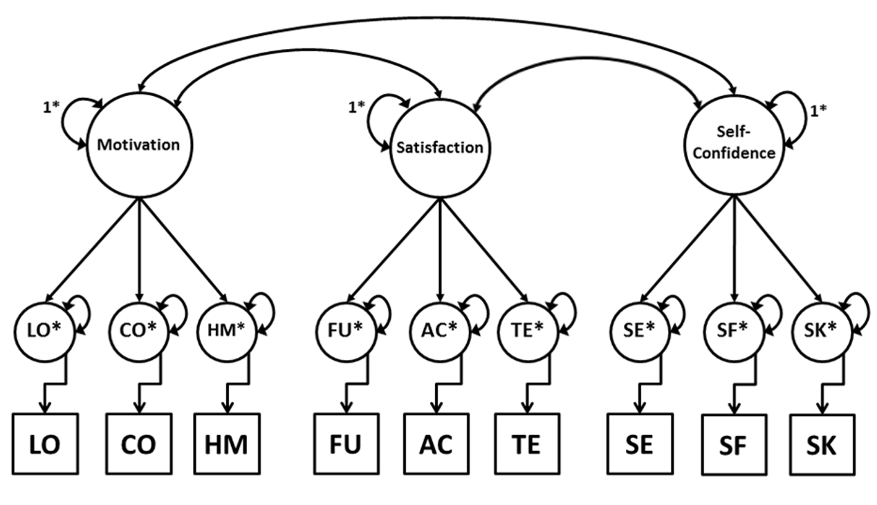
Figure 28.3: Item Factor Analysis (IFA) model of the School Aptitude Questionnaire (SAQ).

Script 28.1

## import raw data
library(foreign)    # the package foreign contains the read.spss function
## create a data frame that contains the data from the spss file saq2cat 
saq2cat <- read.spss("saq2cat.sav", to.data.frame = TRUE)
## extract the variable names from the columns of the saq2cat object
obsnames <- colnames(saq2cat)

## specify the CFA model
modSAQ <- '# factor loadings
    Motivation =~ learning + concentration + homework
    Satisfaction =~ fun + acceptance + teacher
    SelfConfidence =~ selfexpr + selfeff + socialskill
'
## fit model to data 
out.2cat <- cfa(modSAQ, std.lv = TRUE,
                data = saq2cat,        # raw data file
                ordered = obsnames,    # names of ordinal variables
                parameterization = "delta")  # default identification
## results with fit measures and standardized solution
summary(out.2cat, fit = TRUE, std = TRUE)

For the analysis of categorical data it is required that we have the complete raw data file, so that lavaan can calculate the polychoric (here, tetrachoric) correlations. Therefore, we read in the data from an SPSS file “saq2cat.sav” that contains all observed dichotomous responses of all 915 individuals on the SAQ. To do this, we use the read.spss() function that is part of the foreign package. This will result in a data frame saq2cat that has 9 columns (referring to the observed dichotomous variables) and 915 rows (where each row contains the responses of one individual). The names of the variables that are in the SPSS file are used to provide column names for the object saq2cat, and we extract these column names from the saq2cat object to create the obsnames object.

library(foreign)    # the package foreign contains the read.spss function
## create a data frame that contains the data from the spss file saq2cat 
saq2cat <- read.spss("saq2cat.sav", to.data.frame = TRUE)
## extract the variable names from the columns of the saq2cat object
(obsnames <- colnames(saq2cat))

We specify factor loadings for the common factors Motivation, Satisfaction, and Self-Confidence in the lavaan model syntax the same way we did for continuous data. Although the common factors are hypothesized to affect the latent responses $\mathrm{y}^*$ rather than $\mathrm{y}$, we do not need to specify the latent responses in the model syntax. Just like for single-indicator constructs, lavaan will automatically define a latent response for each categorical outcome, giving the latent response the same name as its corresponding observed indicator. We fixed latent variances to 1 with the argument std.lv = TRUE, but as with continuous indicators, we could instead identify common factors by constraining loadings. Likewise, we could constrain intercepts/thresholds instead of common-factor means.

When we fit the model, we use the data= argument to provide the data frame that contains all the observed responses. We do not have to provide separate information on the number of observations or summary statistics of the indicators. In order for lavaan to know which variables are categorical, provide those variable names using the ordered argument.

out.2cat <- cfa(modSAQ, std.lv = TRUE,
                data = saq2cat,              # raw data file
                ordered = obsnames,          # names of ordinal variables
                parameterization = "delta")  # default identification

When lavaan sees that there are ordered outcomes in the model, it will use “DWLS” as the default estimator of model parameters, and it will calculate robust $SE$s and a mean- and variance-adjusted (scaled and shifted) $χ^2$ test statistic in the “Robust” column of the summary() output below (ignore the “DWLS” column, which is the naïve $χ^2$ test statistic).

Number of observations                           915

Estimator                                       DWLS      Robust
  Minimum Function Test Statistic               61.330      86.077
  Degrees of freedom                                24          24
  P-value (Chi-square)                           0.000       0.000
  Scaling correction factor                                  0.731
  Shift parameter                                            2.151
    for simple second-order correction (Mplus variant)

Notice that the “robust” CFI, TLI, and RMSEA values are missing because those have not been worked out yet; the ones in the “Robust” column are merely calculated the naïve way, plugging the $χ^2$ test statistics in the “Robust” column into the standard formulas.

The summary() output contains the usual sections (e.g., factor loadings under “Latent variables”), as well as estimates of the “Thresholds”.

Thresholds:
                   Estimate  Std.Err  z-value  P(>|z|)   Std.lv  Std.all
    learning|t1      -0.796    0.047  -17.076    0.000   -0.796   -0.796
    concentratn|t1   -0.119    0.042   -2.874    0.004   -0.119   -0.119
    homework|t1      -0.322    0.042   -7.619    0.000   -0.322   -0.322
    fun|t1           -1.219    0.055  -22.225    0.000   -1.219   -1.219
    acceptance|t1    -0.881    0.048  -18.410    0.000   -0.881   -0.881
    teacher|t1       -1.091    0.052  -21.060    0.000   -1.091   -1.091
    selfexpr|t1       0.010    0.041    0.231    0.817    0.010    0.010
    selfeff|t1        0.018    0.041    0.430    0.668    0.018    0.018
    socialskill|t1   -0.551    0.044  -12.579    0.000   -0.551   -0.551

Negative threshold values (e.g., “learning | t1”) indicate that the tipping point of scoring “2” instead of “1” is associated with a score of the underlying continuous variable that is below the mean. In other words, it is relatively easy to score “2” on this indicator. A positive value of the threshold indicates that the tipping point of scoring “2” instead of “1” is associated with a score of the underlying continuous variable that is above the mean. Thus, it is relatively difficult to score “2” compared to “1”.

Notice that the standardized solution provides the same values as the unstandardized solution. This is because we used the default method of identifying the latent-response scales (parameterization = "delta"), which is to set their means (actually, their intercepts, because they are endogenous) to zero and their total variances to one. This is indicated in the section “Scales y*:”, which contains the SDs of the latent responses. Notice that they are fixed values, not estimated, so they do not have $SE$s or Wald $z$ tests. Residual variances of latent responses are also not estimated, but are fixed to $θ = 1 − λ^2ψ$, so that the total variance = 1. Recall that we identified the common-factor scale by fixing $ψ = 1$ in this example.

Variances:
                   Estimate  Std.Err  z-value  P(>|z|)   Std.lv  Std.all
   .learning          0.366                               0.366    0.366
   .concentration     0.350                               0.350    0.350
   .homework          0.429                               0.429    0.429
   .fun               0.300                               0.300    0.300
   .acceptance        0.773                               0.773    0.773
   .teacher           0.402                               0.402    0.402
   .selfexpr          0.245                               0.245    0.245
   .selfeff           0.386                               0.386    0.386
   .socialskill       0.607                               0.607    0.607

Scales y*:
                   Estimate  Std.Err  z-value  P(>|z|)   Std.lv  Std.all
    learning          1.000                               1.000    1.000
    concentration     1.000                               1.000    1.000
    homework          1.000                               1.000    1.000
    fun               1.000                               1.000    1.000
    acceptance        1.000                               1.000    1.000
    teacher           1.000                               1.000    1.000
    selfexpr          1.000                               1.000    1.000
    selfeff           1.000                               1.000    1.000
    socialskill       1.000                               1.000    1.000

Thresholds are therefore interpreted as $z$ scores. Likewise, factor loadings are already correlations between the latent common factor and the latent item-response. Because the scaling method is arbitrary, we could have chosen instead to fix the residual variances of the latent responses to be $θ = 1$, so that the total variances would be $1 + λ^2ψ$. This is called the “theta” parameterization, which produces a statistically equivalent model.

The theta parameterization becomes useful when testing hypotheses about equivalence of residual variances, such as strict measurement invariance. In single-group single-occasion models, the choice between delta and theta parameterizations is of little consequence. As Script 28.2 shows, the standardized solution is identical to the unstandardized delta solution.

Script 28.2

## fit the same model to data, using theta parameterization
out.theta <- cfa(modSAQ, std.lv = TRUE, data = saq2cat,
                 ordered = obsnames, parameterization = "theta")
## results with standardized solution
summary(out.theta, std = TRUE)

In this summary() output, the residual variances are now all fixed to 1, and the thresholds are no longer $z$ scores. However, the standardized solution is equivalent to the output above. The $χ^2$ test statistics and fit measures are also unchanged because the delta and theta parameterizations are statistically equivalent (analogous to ULI vs. UVI constraints).

Thresholds:
                   Estimate  Std.Err  z-value  P(>|z|)   Std.lv  Std.all
    learning|t1      -1.315    0.121  -10.904    0.000   -1.315   -0.796
    concentratn|t1   -0.202    0.072   -2.818    0.005   -0.202   -0.119
    homework|t1      -0.491    0.070   -7.024    0.000   -0.491   -0.322
    fun|t1           -2.226    0.327   -6.810    0.000   -2.226   -1.219
    acceptance|t1    -1.002    0.064  -15.695    0.000   -1.002   -0.881
    teacher|t1       -1.720    0.179   -9.613    0.000   -1.720   -1.091
    selfexpr|t1       0.019    0.084    0.231    0.817    0.019    0.010
    selfeff|t1        0.029    0.067    0.429    0.668    0.029    0.018
    socialskill|t1   -0.707    0.062  -11.344    0.000   -0.707   -0.551

Variances:
                   Estimate  Std.Err  z-value  P(>|z|)   Std.lv  Std.all
   .learning          1.000                               1.000    0.366
   .concentration     1.000                               1.000    0.350
   .homework          1.000                               1.000    0.429
   .fun               1.000                               1.000    0.300
   .acceptance        1.000                               1.000    0.773
   .teacher           1.000                               1.000    0.402
   .selfexpr          1.000                               1.000    0.245
   .selfeff           1.000                               1.000    0.386
   .socialskill       1.000                               1.000    0.607

Fixing the latent-response intercepts is also an arbitrary choice. It merely allows us to interpret a threshold between two categories as being a certain distance from the mean, assuming the latent-response mean is zero (controlling for the common factor). But we could just as easily identify the model by fixing the thresholds to zero (an equally arbitrary choice) and estimating the latent-response intercepts. We actually get the same answers but with opposite signs (i.e., $τ = −δ$), which provides the same interpretation. We still interpret a threshold as being a certain distance from the mean of the latent-response distribution, but now we arbitrarily assume the threshold $δ = 0$ instead of assuming the intercept $τ = 0$.

Script 28.3 shows how to specify threshold parameters by using the “|” operator (called a “vertical bar” or “pipe”, found by holding the Shift key and typing the backslash above the Enter/Return key). lavaan always labels thresholds in an orderly fashion, so the first (and only) threshold for a dichotomous response is defined with “| t1”.

Script 28.3

## specify free intercepts and fixed thresholds
mod.fixThresh <- '# factor loadings
  Motivation =~ learning + concentration + homework
  Satisfaction =~ fun + acceptance + teacher
  SelfConfidence =~ selfexpr + selfeff + socialskill
# thresholds for observed variables
  learning | 0*t1
  concentration | 0*t1
  homework | 0*t1
  fun | 0*t1
  acceptance | 0*t1
  teacher | 0*t1
  selfexpr | 0*t1
  selfeff | 0*t1
  socialskill | 0*t1
# intercepts of latent item-responses
  learning ~ NA*1
  concentration ~ NA*1
  homework ~ NA*1
  fun ~ NA*1
  acceptance ~ NA*1
  teacher ~ NA*1
  selfexpr ~ NA*1
  selfeff ~ NA*1
  socialskill ~ NA*1
'
## fit the model to data, using default delta parameterization
out.fixThresh <- cfa(mod.fixThresh, data = saq2cat,
                     std.lv = TRUE, ordered = obsnames)
## results with standardized solution
summary(out.fixThresh, std = TRUE)

In this summary() output, the thresholds are now all fixed to 0, and estimated intercepts have the same values as the previously estimated thresholds, but with opposite signs. Thus, the threshold for “learning” is still 0.796 below the mean of the latent-response distribution, as indicated by the previous estimate of −0.796 (i.e., 0.796 below the fixed intercept of 0). The $SE$s are also of identical magnitude, so Wald $z$ tests yield the same conclusions.

Intercepts:
                   Estimate  Std.Err  z-value  P(>|z|)   Std.lv  Std.all
   .learning          0.796    0.047   17.076    0.000    0.796    0.796
   .concentration     0.119    0.042    2.874    0.004    0.119    0.119
   .homework          0.322    0.042    7.619    0.000    0.322    0.322
   .fun               1.219    0.055   22.225    0.000    1.219    1.219
   .acceptance        0.881    0.048   18.410    0.000    0.881    0.881
   .teacher           1.091    0.052   21.060    0.000    1.091    1.091
   .selfexpr         -0.010    0.041   -0.231    0.817   -0.010   -0.010
   .selfeff          -0.018    0.041   -0.430    0.668   -0.018   -0.018
   .socialskill       0.551    0.044   12.579    0.000    0.551    0.551
    Motivation        0.000                               0.000    0.000
    Satisfaction      0.000                               0.000    0.000
    SelfConfidence    0.000                               0.000    0.000

Thresholds:
                   Estimate  Std.Err  z-value  P(>|z|)   Std.lv  Std.all
    learning|t1       0.000                               0.000    0.000
    concentratn|t1    0.000                               0.000    0.000
    homework|t1       0.000                               0.000    0.000
    fun|t1            0.000                               0.000    0.000
    acceptance|t1     0.000                               0.000    0.000
    teacher|t1        0.000                               0.000    0.000
    selfexpr|t1       0.000                               0.000    0.000
    selfeff|t1        0.000                               0.000    0.000
    socialskill|t1    0.000                               0.000    0.000

To access the polychoric correlation matrix to which the model was fit, use the lavInspect() function. These “observed” polychoric correlations and the model-implied polychorics will both be correlation matrices with diagonals of 1.

> lavInspect(out.2cat, "sampstat") # "observed" tetrachoric correlations
$cov
              lernng cncntr homwrk fun   accptn teachr slfxpr selfff sclskl
learning      1.000                                                        
concentration 0.642  1.000                                                 
homework      0.628  0.585  1.000                                          
fun           0.581  0.399  0.476  1.000                                   
acceptance    0.184  0.238  0.190  0.396 1.000                             
teacher       0.465  0.417  0.380  0.668 0.306  1.000                      
selfexpr      0.335  0.450  0.407  0.241 0.292  0.370  1.000               
selfeff       0.311  0.435  0.373  0.076 0.276  0.151  0.651  1.000        
socialskill   0.141  0.312  0.218  0.071 0.272  0.171  0.548  0.549  1.000
> lavInspect(out.2cat, "cov.ov") # model-implied tetrachoric correlations
             lernng cncntr homwrk fun   accptn teachr slfxpr selfff sclskl
learning      1.000                                                        
concentration 0.642  1.000                                                 
homework      0.602  0.609  1.000                                          
fun           0.467  0.472  0.443  1.000                                   
acceptance    0.265  0.269  0.252  0.398 1.000                             
teacher       0.431  0.437  0.409  0.647 0.368  1.000                      
selfexpr      0.402  0.406  0.381  0.289 0.165  0.267  1.000               
selfeff       0.362  0.367  0.343  0.261 0.148  0.241  0.681  1.000        
socialskill   0.290  0.293  0.275  0.209 0.119  0.193  0.544  0.491  1.000

The Script 28.4 fits the same three-factor model of the SAQ, but now to the raw data of categorical responses with three categories (“1”, “2”, and “3”). With three categories, items now have 2 thresholds (“| t1” and “| t2”). Although specifying factor loadings is sufficient when using thecfa() function because all factor (co)variances and residual variances will be estimated by default, we specify labels for the thresholds in order to illustrate how thresholds can be specified in lavaan model syntax.

Script 28.4

## import 3-category data from the SPSS file saq3cat 
saq3cat <- read.spss("saq3cat.sav", to.data.frame = TRUE)
obsnames <- colnames(saq3cat)
## specify the model
mod.3cat <- '## factor loadings
  Motivation =~ learning + concentration + homework
  Satisfaction =~ fun + acceptance + teacher
  SelfConfidence =~ selfexpr + selfeff + socialskill
## thresholds for observed variables
  learning | th1.1*t1 + th1.2*t2
  concentration | th2.1*t1 + th2.2*t2
  homework | th3.1*t1+ th3.2*t2
  fun | th4.1*t1 + th4.2*t2
  acceptance | th5.1*t1 + th5.2*t2
  teacher | th6.1*t1 + th6.2*t2
  selfexpr | th7.1*t1 + th7.2*t2
  selfeff | th8.1*t1 + th8.2*t2
  socialskill | th9.1*t1 + th9.2*t2
'
## fit the model to data
out.3cat <- cfa(mod.3cat, data = saq3cat,
                std.lv = TRUE, ordered = obsnames)
## results
summary(out.3cat)

The two thresholds for each observed indicator have now been labelled with a suffix (e.g., “th1.1” and “th1.2” for the first and second thresholds of the first item). The output below displays estimated thresholds for the indicators “learning” and “fun”.

Thresholds:
                    Estimate  Std.Err  Z-value  P(>|z|)
    lrnn|1 (t1.1)    -1.224    0.055  -22.269    0.000
    lrnn|2 (t1.2)     0.169    0.042    4.062    0.000
    fun|t1 (t4.1)    -1.563    0.066  -23.580    0.000
    fun|t2 (t4.2)    -0.513    0.044  -11.802    0.000

Interpretation of the thresholds is similar to the situation of dichotomous variables, but now we have information of the threshold for the tipping point of the score “1” to “2”, and of “2” to “3”. So, for the indicator learning it seems that the tipping point of “1” to “2” is associated with a score of the underlying continuous variable below the mean, and that the tipping point of “2” to “3” is associated with a score of the underlying continuous variable above the mean. On the other hand, for the indicator fun both thresholds estimates are negative (and significantly different from zero), which indicates that both tipping points occur for values of the underlying continuous variable that are below the mean. Therefore, it is relatively easy to score high on the indicator fun compared to the indicator learning.

References and further reading

Kamata, A., & Bauer, D. J. (2008). A note on the relation between factor analytic and item response theory models. Structural Equation Modeling, 15(1), 136–153. doi:10.1080/10705510701758406

Mehta, P. D., Neale, M. C., & Flay, B. R. (2004). Squeezing interval change from ordinal panel data: Latent growth curves with ordinal outcomes. Psychological Methods, 9(3), 301–333. doi:10.1037/1082-989X.9.3.301

Muthén, B., & Asparouhov, T. (2002). Latent variable analysis with categorical outcomes: Multiple-group and growth modeling in Mplus: Mplus Web Note 4. Retrieved from http://www.statmodel.com/download/webnotes/CatMGLong.pdf