12 Path Analysis with Categorical Outcomes
Structural equation modeling is a technique designed for continuous variables. In practice, variables are often not continuous but categorical, such as variables scored on discrete Likert scales (i.e., ordinal data) or correct/incorrect responses on test items (i.e., binary data). If endogenous variables in a path model (or in any SEM) are categorical, the SEM-method to deal with the categorical variables is to assume that there exists a latent (unobserved) continuous variable that underlies the observed categorical variable. The underlying variable is called a latent response variable (LRV). Categorical SEM fits the model to the LRVs instead of to the categorical variables. The observed categorical scores can be linked to the LRV using so-called thresholds that represent the value on the LRV beyond which individuals who score higher would get an observed categorical score in the higher category. For example, for a test item that asks ‘How many degrees of freedom does this path model have?’, the students could give the incorrect (scored 0) or the correct (scored 1) answer. The LRV here represents the ability (LRV) to calculate \(df\) for this path model on a continuous scale. Students whose ability is high enough would give the correct response; otherwise, the response would be incorrect. The threshold would reflect the minimum required ability to indicate the correct response. Fitting path models to categorical data thus involves linking the LRV to the observed categorical variables.
In this chapter we first import example data, then we show how one can use probit and logit link functions in a generalized linear model (GLM). Next, we discuss the concept of the LRV for one ordinal variable, for multiple ordinal variables, and then we illustrate fitting a path model to ordinal variables.
12.1 Prepare Data and Workspace
12.1.1 Import Example Data
We will use example data reported by MacKinnon et al. (2007), which are available to download from the Mplus} website} as supplementary materials for a technical report (Muthén, 2011, p. 24). The example data can be downloaded directly from the URL using read.table(file=), as shown below. Note that the data are in summary format (i.e., a table with frequencies for each combination of categories for the 3 variables). The read.table() output is therefore transformed into a standard data.frame with 1 row per subject.
dd <- read.table(file = "http://www.statmodel.com/examples/shortform/4cat%20m.dat",
                 col.names = c("intention", "intervention", "ciguse", "w"))
dd$intention <- dd$intention - 1L # make the lowest category 0, not 1
## transform frequency table to casewise data
myData <- do.call(rbind, lapply(1:nrow(dd), function(RR) {
    data.frame(rep(1, dd$w[RR]) %*% as.matrix(dd[RR, 1:3]))
}))- Predictor:
intervention(1 = treatment, 0 = control) - Mediator:
intentionto smoke in the following 2 months (measured 6 months after intervention)- 0 = No, 1 = I don’t think so, 2 = Probably, 3 = Yes
- Outcome:
cigusein previous month (1 = smoked, 0 = not), measured a 1-year follow-up
12.1.2 Summarize Data
The resulting data.frame looks like this:
##     intention intervention ciguse
## 415         0            1      0
## 463         0            1      0
## 179         1            0      1
## 526         0            1      0
## 195         1            0      0
The marginal frequencies for each variable are:
## $intention
##
##   0   1   2   3
## 644 103  60  57
##
## $intervention
##
##   0   1
## 371 493
##
## $ciguse
##
##   0   1
## 708 156
Let’s begin with a frequency table to estimate the proportion of subjects who smoke cigarettes (i.e., the estimated probability of smoking: \(\widehat{\pi}\)) in each combination of categories for the predictors.
## Margins computed over dimensions
## in the following order:
## 1: intention
## 2: intervention
## intervention
## intention 0 1 mean
## 0 0.11583012 0.08311688 0.09947350
## 1 0.26530612 0.20370370 0.23450491
## 2 0.58823529 0.42307692 0.50565611
## 3 0.68965517 0.67857143 0.68411330
## mean 0.41475668 0.34711723 0.38093696The treatment group (intervention == 1) smokes less, both on average and within each intention group. Smoking also increases with intent to smoke (both on average and within treatment/control groups). Treatment appears least effective among those who were certain they would continue smoking (row 4).
12.2 Regression Models for Binary Variables
Suppose we used a linear model to predict the probability of smoking, treating intention as a continuous predictor to estimate only its linear effect.
##  (Intercept) intervention    intention
##    0.1177588   -0.0439528    0.1927033
The estimated intercept indicates the predicted probability of smoking when predictors are zero (i.e., those in the control group with no intent to smoke). The estimated slopes reflect what we saw in the table: treatment reduces the probability of smoking (given the intent to smoke), and intent to smoke is associated with more smoking (given treatment).
- Note: No interaction is included here, but you can test for yourself that it was not significant.
It would be problematic if the model predicted any probabilities outside the natural 0–1 range. We do not observed that problem in this specific sample:
##    Min. 1st Qu.  Median    Mean 3rd Qu.    Max.
## 0.07381 0.07381 0.11776 0.18056 0.26651 0.69587
This limitation of linear probability models is resolved with a link function in a GLM that allows for predicted values along the entire real-number line. Two such transformations are in frequent use:
- The probit (probability unit) transformation dates back to Bliss (1934). A probability can be transformed to a corresponding quantile in a cumulative distribution function (CDF), such as the standard-normal distribution. In other words, any probability \(p\) between 0–1 has a corresponding \(z\) score, such as can be requested from
qnorm(p). Likewise, any predicted value on the probit scale can be transformed back into a probability usingpnorm(probit). The GLM takes the form below, where \(\Phi()\) is the standard-normal CDF, \(\Phi^{-1}()\) is its inverse, and \(\mathbf{XB}\) is the linear predictor (\(\widehat{y}\)):
\[ \text{Probit}(y=1) = \Phi(\pi) = z = \mathbf{XB} \]
\[ \text{Pr}(y=1) = \pi = \Phi^{-1}(z) \]
- The logit (logistic unit) transformation is often favored because its coefficients can be interpreted on the (natural-)log-odds scale. Recall the odds of an outcome is a ratio of its probability (\(\pi\)) to its complement (\(1-\pi\)), so its range is 0 to \(+\infty\) (i.e., it is merely bound to nonnegative numbers). The natural (i.e., base-\(e\)) log of a nonnegative number can take any real number. The formulas below show how probabilities, odds, and logits are related.
\[ \text{Logit}(\pi) = \ln(\text{odds}) = \ln \Bigg(\frac{\pi}{1 - \pi} \Bigg) = \mathbf{XB} \]
\[ \text{odds} = \frac{\pi}{1 - \pi} = \mathrm{e}^{\text{Logit}(\pi)} \text{ , where } \; \; \mathrm{e} = 2.7182818 \]
\[ \pi = \frac{\text{odds}}{1 + \text{odds}} = \frac{\mathrm{e}^\text{Logit}}{1 + \mathrm{e}^\text{Logit}} \]
There is a logit() function in the psych package, but it is simple enough to calculate the transformation (and its inverse):
logit <- log( p / (1-p) )           # odds <- p / (1-p)
p <- exp(logit) / (1 + exp(logit))  # odds <- exp(logit)
Both probit and logistic regression models can be estimated using the glm() function, demonstrated below.
12.2.1 Fit a Logistic Regression Model
In order to compare the results of fitting the logistic and the probit regression models, we first fit the GLM with the logit link. We continue to treat the ordinal mediator intention as continuous for now.
mod.logit <- glm(ciguse ~ intervention + intention, data = myData,
                 family = binomial("logit"))
coef(mod.logit)
## (Intercept) intervention intention
## -2.0177349 -0.3771387 1.037973312.2.2 Fit a Probit Regression Model
mod.probit <- glm(ciguse ~ intervention + intention, data = myData,
                  family = binomial("probit"))
coef(mod.probit)
## (Intercept) intervention intention
## -1.1894765 -0.2030216 0.608151212.2.3 Compare Models
The GLMs make very similar predictions. We can compare all 3 models’ (linear, logit and probit) predictions to the observed probabilities in each group.
##    intention intervention      p.obs   p.linear    p.logit   p.probit
## 1          3            1 0.67857143 0.65191604 0.67239696 0.66711311
## 3          3            0 0.68965517 0.69586883 0.74954459 0.73727830
## 5          2            1 0.42307692 0.45921270 0.42093726 0.43007009
## 7          2            0 0.58823529 0.50316549 0.51454880 0.51070069
## 9          1            1 0.20370370 0.26650936 0.20474455 0.21641830
## 11         1            0 0.26530612 0.31046215 0.27293908 0.28051061
## 13         0            1 0.08311688 0.07380601 0.08356445 0.08188581
## 15         0            0 0.11583012 0.11775881 0.11735341 0.11712611
Notice how similar the predicted probabilities are across models, and how close they are to the observed proportions in each group.
Each of these models estimates the same number of parameters, but their functional form differs (identity, logit, and probit link functions, with different models for error). So we can only compare the fit of each model to the data descriptively. Here are two examples: (1) sum the squared differences between each model’s predicted probabilities and the observed probabilities, summarized by Pearson’s \(\chi^2\) statistic (lower fits better):
##   p.linear    p.logit   p.probit
## 0.04094642 0.01564608 0.01676192
Or compare their Tjur’s pseudo-\(R^2\) values (higher fits better):
##    linear     logit    probit
## 0.2042811 0.2074272 0.2063500
In both cases, the logit model performs slightly better than probit, both of which perform better than the linear model. But the discrepancies are small.
12.3 Latent Response Variable
In SEM, the probit model is often preferred because predicted values are \(z\) scores that can be transformed into probabilities. This lends itself easily to a latent-response interpretation, which can be stated as follows for the cigarette-use example.
- Each subject has a latent propensity to smoke. This propensity is a continuous, normally distributed trait. Subjects whose propensity exceeds a threshold succumb to smoking, whereas those whose propensity does not exceed the threshold refrain from smoking.
The probit model above can therefore be reframed in terms of this LRV, \(\mathrm{y}^*\).
\[\mathrm{y}^* = \mathbf{XB} + \varepsilon ,\] where \(\varepsilon \sim \mathcal{N}(0, \sigma)\) and the observed binary response \(\mathrm{y}\) is linked to the LRV by a threshold model:
\[\mathrm{y} = I(y^* > \tau),\]
where the indicator function \(I()\) assigns 1 when its argument is TRUE and 0 when it is FALSE. Because the LRV is unobserved (i.e., latent), its distributional parameters cannot be estimated from the data. GLM software like the glm() function typically identify the model by fixing the residual variance \(\sigma=1\) and the threshold \(\tau=0\). For simplicity, consider an intercept-only model for cigarette use.
## (Intercept)
##  -0.9132499
In lavaan the default is instead to fix the intercept to 0 and estimate the threshold. The model syntax below shows how thresholds are specified with the “pipe” (vertical bar: |) followed by t1 indicating the first threshold.
mod0.ciguse <- 'ciguse | t1' # specify first (and only) threshold
fit0.ciguse <- sem(mod0.ciguse, data = myData)
summary(fit0.ciguse, header = FALSE, nd = 7)
##
## Parameter Estimates:
##
## Parameterization Delta
## Standard errors Robust.sem
## Information Expected
## Information saturated (h1) model Unstructured
##
## Thresholds:
## Estimate Std.Err z-value P(>|z|)
## ciguse|t1 0.9132499 0.0498031 18.3372246 0.0000000
##
## Variances:
## Estimate Std.Err z-value P(>|z|)
## ciguse 1.0000000Binary variables have only 1 threshold that splits a normal distribution into 2 categories. Notice that it is arbitrary whether the intercept (mean) or threshold is fixed to 0.
- In the output of
glm()the threshold was fixed at zero and intercept was estimated to be \(-0.913\). - In the output of
lavaanthe intercept is fixed at zero and the threshold was estimated to be \(+0.913\).
In either case, the threshold is the same distance from the LRV’s mean, as depicted in Figure 12.1 below.
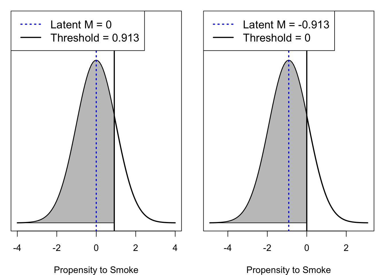
Figure 12.1: One threshold divides a normal distribution into two categories.
Notice that the distributions are identical. Only the \(x\)-axis differs, reflecting the change in (arbitrary) identification constraint.
12.3.1 Ordinal Outcomes
The LRV interpretation is easily extended to polytomous ordinal variables, such as intent to smoke. This is called the cumulative probit model (and link function). Any ordinal variable with categories \(c=0, \ldots, C\) can be interpreted as a crude discretization of an underlying LRV, whose \(C\) thresholds divide the latent distribution into \(C+1\) categories.
\[\mathrm{y}=c \ \ \ \text{ if } \ \ \ \tau_c < y^* \le \tau_{c+1} \]
Because the normal distribution is unbounded, the first category “starts” at \(\tau_0 = -\infty\), and the last category “ends” at \(\tau_{C+1} = +\infty\). For example, intent to smoke has 4 categories, so there are \(C=3\) thresholds. We do not have to specify thresholds in lavaan model syntax if we tell lavaan which variables are ordinal using the argument ordered=. When all modeled variables are ordinal, one can use TRUE as a shortcut.
fit2 <- sem('ciguse ~~ intention', data = myData, ordered = TRUE)
summary(fit2, header = FALSE, standardized = TRUE)
##
## Parameter Estimates:
##
## Parameterization Delta
## Standard errors Robust.sem
## Information Expected
## Information saturated (h1) model Unstructured
##
## Covariances:
## Estimate Std.Err z-value P(>|z|) Std.lv Std.all
## ciguse ~~
## intention 0.637 0.041 15.496 0.000 0.637 0.637
##
## Thresholds:
## Estimate Std.Err z-value P(>|z|) Std.lv Std.all
## ciguse|t1 0.913 0.050 18.337 0.000 0.913 0.913
## intention|t1 0.660 0.046 14.280 0.000 0.660 0.660
## intention|t2 1.101 0.054 20.570 0.000 1.101 1.101
## intention|t3 1.506 0.066 22.867 0.000 1.506 1.506
##
## Variances:
## Estimate Std.Err z-value P(>|z|) Std.lv Std.all
## ciguse 1.000 1.000 1.000
## intention 1.000 1.000 1.000Notice that intent has 3 thresholds, labeled with sequential integers following the letter t. This is how they would be specified in lavaan model syntax, e.g.,
Alternatively, set the argument auto.th=TRUE to automatically estimate all thresholds.
The LRV for intention can be interpreted as the degree to which someone intends to smoke—similar to the observed variable, but the degree increases continuously rather than in discrete increments.
- Subjects in Category 0 do not have a latent intent to smoke that exceeds the first threshold (\(\hat\tau_1\)), so they do not indicate that they intend to smoke.
- Subjects will only respond that they “don’t know” when their latent intent exceeds \(\hat\tau_1=\) 0.66 \(SD\)s above the mean of that distribution.
- Subjects must exceed \(\hat\tau_2=\) 1.101 \(SD\) above the mean before they begin indicating “probably”.
- Only those whose latent intent exceeds \(\hat\tau_3=\) 1.506 \(SD\)s above the mean do they respond firmly “yes”.
Figure 12.2 below visualizes the “classification rules” above.
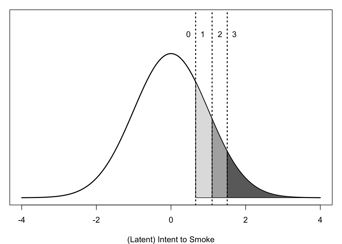
Figure 12.2: Three thresholds divide a normal distribution into four categories.
12.3.2 Estimating Thresholds
Thresholds are univariate statistics (like means). Threshold estimates are based on the frequency distribution of a categorical variable. Recall that the probit function merely transforms a (predicted) probability (\(\pi\)) into a corresponding \(z\) score. The (standardized) thresholds are these \(z\) scores. We can estimate them by plugging into qnorm() the cumulative proportions (\(\widehat\pi_c\)) up to each category \(c\). For example, here are the (cumulative) proportions in each category of intention.
p.intent <- prop.table(table(myData$intention)) # proportions per category
cumsum(p.intent) # cumulative proportions (up to and including each category)
## 0 1 2 3
## 0.7453704 0.8645833 0.9340278 1.0000000By definition, 100% of the sample was observed in any of the categories up to (and including) the highest category, so the final cumulative proportion is 1. Likewise, no one in the sample was observed in a category lower than the lowest category (by definition), so we can append a zero as the first number in this vector of cumulative proportions. Then we can find the corresponding \(z\) scores in a normal distribution, which are the thresholds between categories:
##                   0         1         2         3
##      -Inf 0.6599915 1.1011455 1.5064783       Inf
The upper and lower thresholds are \(+/-\infty\) by definition, corresponding to 0 and 100%. Those never need to be estimated because they are fixed by design. The remaining 3 thresholds are actual borders between observed categories, showing how far above/below the mean a subject must be in order to indicate a particular response category.
12.3.3 Estimating Polychoric Correlations
With multiple ordinal variables, we can estimate the correlations between their associated LRVs by relying on the assumption that the LRVs are normally distributed (Olsson, 1979, 1982). These correlations are called polychoric correlations (Olsson, 1979), which are bivariate statistics (like the covariance matrix). If the model also includes a continuous variable, its correlation with an ordinal variable’s LRV is called the polyserial correlation (Olsson, 1982). Special names for 2-category variables are tetrachoric correlation (between 2 binary variables) or biserial correlation (between a binary and continuous variable). For example, the estimated covariance between cigarette use and intent to smoke in the model above is a polychoric correlation because each LRV’s \(SD\) was fixed to 1 in that unrestricted (saturated) model.
The reason that the probit model is so popular in SEM is that the standard SEM matrices and interpretations still apply to normal data, except those normal variables are latent. All we need to do is append the SEM with a threshold model in order to link these normal LRVs to their observed discrete counterparts. The default saturated model in lavaan estimates all thresholds and polychoric (and polyserial, if applicable) correlations, along with means and (co)variances among any continuous variables. This is used as input data when fitting any hypothesized model (even when fitting a regression model with \(df=0\)). We can see the estimated sample statistics for the model above:
## $cov
##           ciguse intntn
## ciguse     1.000
## intention  0.637  1.000
##
## $mean
##    ciguse intention
##         0         0
##
## $th
##    ciguse|t1 intention|t1 intention|t2 intention|t3
##        0.913        0.660        1.101        1.506
Notice that the means are 0 and variances are 1, consistent with the correlation metric and the assumption that the underlying LRV is a \(z\) score. These values are actually fixed to identify the saturated model. We will discuss scaling constraints and identification of latent variables more when we introduce the common-factor model.
12.3.4 Estimating an SEM with Estimated Input
The problem with treating thresholds and polychoric correlations as observed data is that they were not observed. They are estimates of population parameters, based on the data. They each have an associated \(SE\) and 95% CI. In order to trust the \(SE\)s, 95% CIs, and test statistics in our hypothesized model, we need to take the uncertainty of the “data” into account. This is often accomplished using weighted least-squares estimation, where the weight matrix \(\mathbf{W}\) is the sampling covariance matrix of the estimated thresholds and polychoric correlations.
- Note: Do not confuse the sampling covariance matrix of estimated parameters with the covariance matrix of variables. The latter is used as input data, and it is what we want our SEM to explain. The sampling covariance of parameter estimates is how we quantify their uncertainty: its diagonal contains sampling variances, the square-roots of which are the \(SE\)s that we use to calculate Wald \(z\) tests and CIs.
The more variables (and categories) there are, the larger \(\mathbf{W}\) becomes: there is one row/column for every estimated threshold and correlation. Even in samples as large as 1000, this makes estimation unstable. An alternative is to simply ignore the sampling covariances during estimation, so \(\text{diag}(\mathbf{W})\) is the weight matrix to obtain point estimates of parameters. This is called diagonally weighted least squares (estimator = "DWLS"), which is the default in lavaan. Even with DWLS, the full weight matrix is still needed to calculate \(SE\)s and the \(\chi^2\) statistic. The \(\chi^2\) statistic needs to be robust against the uncertainty of the input data, so it is adjusted by scaling it (a mean-adjusted statistic) and optionally shifting it (a mean- and variance-adjusted statistic). The default is both: estimator = "WLSMV" is a shortcut that implies
lavaan(..., estimator = "DWLS", se = "robust.sem", test = "scaled.shifted")
Another alternative is unweighted/ordinary least squares (ULS), where \(\mathbf{W}\) is an identity matrix. This often yields good point estimates, but Type I error rates can differ from the \(\alpha\) level, so it is still recommended to request a scaled/shifted \(\chi^2\) statistic (e.g., estimator = "ULSMV").
There are also likelihood-based estimators. One option is marginal maximum likelihood (estimator = "MML"), which is currently disabled in lavaan because it was too computationally intensive and the developer is exploring better routines. A less computationally intensive alternative is pairwise maximum likelihood (estimator = "PML"), which maximizes only the (sum of) uni- and bivariate (log-)likelihoods. This is a quite robust procedure even in small samples, and because it is likelihood-based, information criteria (AIC and BIC) are available.
Note: The “robust” statistics are only corrected for the two-stage estimation procedure (thresholds+pollychorics, followed by SEM parameters using DWLS or ULS) or for combining pairwise log-likelihoods (using PML). The LRV interpretation for categorical outcomes assumes a normal distribution for latent responses. Because LRVs are (by definition) unobserved, there is no way to estimate their degree of nonnormality, which would be necessary to correct for it.
12.3.4.1 Counting Degrees of Freedom
For SEM with only continuous variables, the number of observed summary statistics \(p^*\) is a simply function of the number of variables \(p\):
\[p^* = \frac{p(p+3)}{2} \text{ (with mean structure) or } \frac{p(p+1)}{2} \text{ (without means)}\]
- \(p\) means
- \(p\) variances
- \(\frac{p(p-1)}{2}\) covariances
The number of “observed” covariances does not differ between continuous and categorical variables, but some covariances are replaced by:
- polychoric correlations among LRVs
- (scaled) polyserial correlations between LRVs and observed variables
But the number of univariate statistics can differ. Whereas continuous variables each contribute an observed mean and variance, categorical variables do not contribute either (i.e., those values are fixed to 0 and 1, respectively, to estimate thresholds and polychoric correlations). Instead, each categorical variable contributes \(C\) “observed” standardized thresholds for its \(C+1\) categories. So each binary variable contributes \(C=1\) threshold, each “ternary” (3-category) variable contributes \(C=2\) thresholds, and so on. Thus, the number summary statistics is a function of the number of observed continuous and discrete variables. Suppose we denote:
- \(p_c\) the number of continuous variables
- \(p_d\) the number of discrete variables
- so the total number of observed variables remains \(p = p_c + p_d\)
- the number of thresholds for discrete variables \(d = 1, \dots, D\) is \(C_d\)
- the total number of thresholds is \(K = \sum_{d=1}^D C_d\)
Then the number summary statistics is \(\frac{p(p-1)}{2} + 2p_c + K\). That is, both continuous and discrete variables contribute covariances/correlations (first term), only continuous variables contribute a mean and variance (second term), and only discrete variables contribute thresholds (third term).
This has implications for determining the expected \(df\), which is an important part of verifying that you fit the model you intended to fit. Just as mean structures are typically saturated (e.g., for every observed mean, an intercept is estimated), each “observed” standardized threshold has a corresponding estimated threshold (not necessarily standardized, but is by default in lavaan). Likewise, intercepts and (residual or marginal) variances typically remain fixed for LRVs in hypothesized models, as they do in the default saturated model. Thresholds might be constrained (contributing \(df\)) in models for multiple groups or occasions—as might LRV intercepts or (residual or marginal) variances—which we discuss in later chapters.
12.3.4.2 Missing Data
When multivariate-normal data are incomplete, all available information can be used to estimate parameters by setting missing = "FIML" (full-information ML estimation) to override the default listwise deletion method. Actually, FIML applies to nonnormal continuous data as well, since a robust correction for nonnormality is available with FIML results (estimator = "MLR"). FIML is also available for categorical outcome(s), but only when using (marginal) ML estimation. Until estimator = "MML" becomes available in lavaan, the FIML option is unfortunately unavailable.
When at least 1 endogenous variable is binary/ordinal, missing = "pairwise" deletion retains as much information as possible, so it is still preferred over the default missing = "listwise" deletion. However, both deletion methods make the restrictive assumption that data are missing completely at random (MCAR). The reason pairwise deletion assumes MCAR data is that for each pair of variables, it estimates their covariance (or polychoric/polyserial correlation) using all jointly observed complete data for that pair of variables. So no information from other observed variables can be used to estimate the covariance/correlation.
In contrast, FIML estimates parameters using each person’s entire vector of observed data, so missing data on Variable A can be compensated by observed data on Variable B. Thus, FIML makes the less restrictive assumption that data are missing at random (MAR)—that is, the missingness is still random conditional on the observed data (see Little et al., 2014, for more detailed conceptual explanations).
Pairwise deletion is available with any (diagonally or un)weighted least-squares estimators, as well as with (P)ML. But with PML for categorical outcomes, a missing = "doubly.robust" estimation method is available that only requires assuming data are MAR (Katsikatsou et al., in press). It is computationally intensive, but it may be worth it if the MAR assumption is not feasible.
12.4 Mediation Model with Categorical Outcomes
Consider the mediation model depicted in Figure 12.3 below. The dashed line is the direct effect of treatment on smoking behavior, given the intent to smoke.
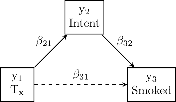
Figure 12.3: Mediation model for smoking-intervention data from Duncan and Duncan (1996).
Because SEM treats an exogenous binary predictor as numeric (like dummy-coded predictors in standard OLS regression models), these \(p=3\) variables include \(p_c=1\) “continuous” predictor (intervention) and \(p_d=2\) discrete outcomes. These contribute \(p^* = \frac{p(p-1)}{2} = 3\) “observed” covariances:
- The polyserial correlations of
interventionwithciguseandintention - The polychoric correlation between
ciguseandintention
The predictor also contributes \(2p_c=2\) observed values: a mean and a variance. The endogenous binary variable ciguse contributes 1 threshold, and the endogenous ordinal variable intention contributes 3 thresholds, so \(K=4\). Thus, there are 3 + 2 + 4 = 9 summary statistics in this 3-variable system.
There are 3 possible conclusions:
- No mediation: the indirect effect \(\beta_{21} \times \beta_{32}=0\) because either \(\beta_{21}=0\) or \(\beta_{32}=0\)
- Partial mediation: the indirect effect \(\beta_{21} \times \beta_{32} \ne 0\) and the direct effect \(\beta_{31} \ne 0\)
- Full mediation: the indirect effect \(\beta_{21} \times \beta_{32} \ne 0\) but the direct effect \(\beta_{31} = 0\)
Omitting the dashed line (by fixing \(\beta_{31}=0\)) would imply full mediation. A full-mediation model would estimate 8 parameters:
- 2 regression slopes (\(\beta_{21}\) and \(\beta_{32}\))
- 1 mean and 1 variance for the exogenous dummy coded
intervention - 3 thresholds for the mediator
intention - 1 threshold for the outcome
ciguse
Thus, the full-mediation model will have \(df=1\). The partial-mediation model would estimate the dashed line, reducing \(df=0\). No mediation could be represented by a model that estimates the dashed line but fixes either \(\beta_{21}=0\) (a multiple-regression model for ciguse) or \(\beta_{32}=0\) (a multivariate regression model for intention and ciguse). We will only fit the full and partial mediation models in the next section.
12.4.1 Estimate Mediation Models
Begin by fitting the partial-mediation model to the data, to test \(H_0: \beta_{21} \times \beta_{32}=0\) (no mediation). We will only specify the regression slopes and user-defined parameters because the residual variances are not estimated. The identification constraints require more explanation (see the following section).
mod.part <- ' ## regression paths
    intention ~ b21*intervention
    ciguse ~ b31*intervention + b32*intention
  ## define indirect and total effects
    ind := b21*b32
    tot := ind + b31
'
fit.part <- sem(mod.part, data = myData, ordered = TRUE)
summary(fit.part, standardized = TRUE, rsquare = TRUE)
## lavaan 0.6-20.2318 ended normally after 13 iterations
##
## Estimator DWLS
## Optimization method NLMINB
## Number of model parameters 7
##
## Number of observations 864
##
## Model Test User Model:
## Standard Scaled
## Test Statistic 0.000 0.000
## Degrees of freedom 0 0
##
## Parameter Estimates:
##
## Parameterization Delta
## Standard errors Robust.sem
## Information Expected
## Information saturated (h1) model Unstructured
##
## Regressions:
## Estimate Std.Err z-value P(>|z|) Std.lv Std.all
## intention ~
## intrvntn (b21) -0.246 0.089 -2.758 0.006 -0.246 -0.121
## ciguse ~
## intrvntn (b31) -0.130 0.093 -1.402 0.161 -0.130 -0.064
## intentin (b32) 0.631 0.042 15.105 0.000 0.631 0.629
##
## Thresholds:
## Estimate Std.Err z-value P(>|z|) Std.lv Std.all
## intention|t1 0.525 0.067 7.844 0.000 0.525 0.521
## intention|t2 0.970 0.071 13.572 0.000 0.970 0.963
## intention|t3 1.378 0.082 16.710 0.000 1.378 1.368
## ciguse|t1 0.760 0.072 10.491 0.000 0.760 0.752
##
## Variances:
## Estimate Std.Err z-value P(>|z|) Std.lv Std.all
## .intention 1.000 1.000 0.985
## .ciguse 0.602 0.602 0.591
##
## R-Square:
## Estimate
## intention 0.015
## ciguse 0.409
##
## Defined Parameters:
## Estimate Std.Err z-value P(>|z|) Std.lv Std.all
## ind -0.155 0.057 -2.713 0.007 -0.155 -0.076
## tot -0.285 0.100 -2.845 0.004 -0.285 -0.140Using the standard criterion \(\alpha=5\%\), the Wald \(z\) tests allow us to reject the \(H_0\) of no mediation: indirect effect \(b\) = \(-0.155\), \(z = -2.713\), p = 0.007, \(\beta = -0.076\). We fail to reject the \(H_0\) of full mediation: direct effect b = \(-0.13\), \(z = -1.402\), p = 0.161, \(\beta = -0.064\).
Because the scales of the LRVs are arbitrary, it is safer to
- interpret the standardized slopes
- test a \(H_0\) using a \(\Delta \chi^2\) test
We can fit a full-mediation model to the data to obtain the LRT.
mod.full <- ' ## regression paths
    intention ~ b21*intervention
    ciguse ~ b32*intention
  ## define indirect and total effects
    ind := b21*b32
'
fit.full <- sem(mod.full, data = myData, ordered = TRUE)
lavTestLRT(fit.full, fit.part) # or anova(), which then calls lavTestLRT()
##
## Scaled Chi-Squared Difference Test (method = "satorra.2000")
##
## lavaan->lavTestLRT():
## lavaan NOTE: The "Chisq" column contains standard test statistics, not the
## robust test that should be reported per model. A robust difference test is a
## function of two standard (not robust) statistics.
##
## Df AIC BIC Chisq Chisq diff Df diff Pr(>Chisq)
## fit.part 0 0.0000
## fit.full 1 1.2648 1.9567 1 0.1619Notice that lavTestLRT() automatically detects the robust estimator and test statistic requested when fitting the models, so it appropriately uses the same robust correction (mean- and variance-adjustment) for the \(\Delta \chi^2\) statistic. This is why the Chisq Diff column does not match the difference between (uncorrected) \(\chi^2\) values in the Chisq column. The \(p\) value is very close to the Wald test’s \(p\) value (also calculated using a robust \(SE\)), which is expected when \(N\) is large.
12.4.2 Interpreting Coefficients
Notice that the glm() estimates from the probit regression for ciguse do not match those from the sem() function. There are noteworthy differences in parameterization:
- The GLM approach fixes the threshold to 0 and estimates the intercept. The SEM approach fixes the intercept to 0 and estimates the threshold. As shown in the figure above, this distinction is arbitrary because the LRV has no “location” that we can identify from the data. The intercept and threshold can only be said to be a certain distance apart, which is why they take the same absolute value. For example, we can free the
ciguseintercept inlavaansyntax and fix its threshold instead:
## ciguse|t1  ciguse~1
## 0.7596909 0.0000000
## fixed threshold
mod.trade <- ' ciguse | 0*t1 # fix threshold
ciguse ~ NA*1 # estimate intercept '
coef(sem(c(mod.part, mod.trade), data = myData, ordered = TRUE),
type = "all")[c("ciguse|t1","ciguse~1")]## ciguse|t1 ciguse~1
## 0.0000000 -0.7596909- The GLM approach treats all predictors as fixed, and predictors are distinct from outcomes. Intent to smoke was treated as continuous. Although we could have used polynomial contrast codes to estimate linear, quadratic, and cubic effects, we still would have to take the observed category weights (0–3) as given.
- The SEM approach allows outcomes to predict other outcomes. So the LRV underlying intent to smoke was used as a predictor of smoking propensity (LRV underlying
ciguse). This allows us to extrapolate from our results what we would expect if we had measured intent as a continuous variable (and it happened to be normally distributed).
A final distinction has to do with the identification constraint on the LRV scale.
12.4.3 Delta vs. Theta Parameterizations
The SEM approach in lavaan (by default) fixes the marginal (i.e., total) variance of the LRV to 1. This is called the “delta parameterization” in the SEM literature. The GLM approach fixes the residual/conditional variance to 1. This is called the “theta parameterization” in the SEM literature.
Under the delta parameterization, the residual variance is fixed such that it equals 1 minus the explained variance (\(1-R^2\)). Under the theta parameterization, the LRV’s total variance is the sum of explained and unexplained variance (1 + explained variance). The total variances is not an explicit SEM parameter; instead, the scaling factors (Scales y* in the output) are the reciprocal of the total \(SD\) (i.e., \(\frac{1}{SD}\)).
Use the argument parameterization = "theta" to override the default delta parameterization, if there is a reason to do so (i.e., if you want to model residual variances). This will be discussed further in the chapter about item factor analysis (i.e., common-factor models for categorical indicators).
This arbitrary distinction can have important consequences for the interpretation and decomposition of mediated effects. For example, the indirect effects would not be comparable between full- and partial-mediation models when fixing residual variances to 1, because doing so would change the scale of the LRV across the two models. That is, the relative amount of residual variance would be different for the full- and partial mediation models. The partial-mediation model explains less variance (lower \(R^2\), so its residual variance should be larger) than the full-mediation model, but residual variances are fixed to 1 in both cases, making the total variance appear smaller in the partial-mediation model. This change of scales changes the meaning of ‘one unit increase’ across the models.
Luckily, when using the delta parameterization in single-group models, the outcome’s LRV scale (and any categorical mediator’s LRV scale) is already held constant by fixing the marginal variance to 1 (Breene et al., 2013). However, this good news would not apply in more complex situations that affect LRV scales, such as multigroup models. So when using path analysis with categorical outcomes, it is best to exercise caution. Use the delta parameterization, and do not use a multigroup models to compare paths across groups (i.e., moderated mediation) unless you understand how to equate the LRV scales across groups.
12.4.4 Decomposing Total Effects
Furthermore, a common method of quantifying the size of an indirect effect is the proportion of the total effect: \(\frac{\beta_{21} \times \beta_{32}}{(\beta_{21} \times \beta_{32}) + \beta_{31}}\). This is already problematic when the direct and indirect effects have opposite signs (called inconsistent mediation). But when the scale of a LRV varies between models with(out) a mediator, then the sum of estimated direct and indirect effects would no longer match the total effect.
For example, fit separate probit models for the mediator and outcome, as would be necessary using the GLM approach. For simplicity, only treat ciguse as categorical.
## simple regression to obtain the total effect
(total <- coef(sem('ciguse ~ total*intervention', data = myData,
                   ordered = 'ciguse', parameterization = "theta"))["total"])
## total
## -0.2850428## b21
## -0.1644697## model for outcome
(b3 <- coef(sem('ciguse ~ b31*intervention + b32*intention', data = myData,
ordered = 'ciguse', parameterization = "theta"))[c("b31","b32")])## b31 b32
## -0.2030216 0.6081512## b21
## -0.303044This does not match the total effect from the simple probit regression because the LRV scales differ. That is, the simple regression has more residual variance (less explained variance without intention in the model), yet the residual variance is still fixed to 1. Imai et al. (2010) proposed a general solution to this problem, using the causal-modeling framework, implemented in the mediation (see their `vignette for examples). It is quite complicated, but here is how it would apply to our current example (see also Muthén, 2011, for corresponding Mplus syntax):
mod.Imai <- '
    ciguse ~ c*intervention + b*intention
    intention ~ a*intervention
# label threshold for ciguse
    ciguse | b0*t1
# biased SEs
    naive.indirect := a*b
    naive.direct := c
# correct
    probit11 := (-b0+c+b*a)/sqrt(b^2+1)
    probit10 := (-b0+c )/sqrt(b^2+1)
    probit00 := (-b0 )/sqrt(b^2+1)
    indirect := pnorm(probit11) - pnorm(probit10)
    direct := pnorm(probit10) - pnorm(probit00)
'
fit <- sem(mod.Imai, data = myData, ordered = c("ciguse","intention"))
summary(fit, std = TRUE)
## lavaan 0.6-20.2318 ended normally after 13 iterations
##
## Estimator DWLS
## Optimization method NLMINB
## Number of model parameters 7
##
## Number of observations 864
##
## Model Test User Model:
## Standard Scaled
## Test Statistic 0.000 0.000
## Degrees of freedom 0 0
##
## Parameter Estimates:
##
## Parameterization Delta
## Standard errors Robust.sem
## Information Expected
## Information saturated (h1) model Unstructured
##
## Regressions:
## Estimate Std.Err z-value P(>|z|) Std.lv Std.all
## ciguse ~
## interventn (c) -0.130 0.093 -1.402 0.161 -0.130 -0.064
## intention (b) 0.631 0.042 15.105 0.000 0.631 0.629
## intention ~
## interventn (a) -0.246 0.089 -2.758 0.006 -0.246 -0.121
##
## Thresholds:
## Estimate Std.Err z-value P(>|z|) Std.lv Std.all
## ciguse|t1 (b0) 0.760 0.072 10.491 0.000 0.760 0.752
## intntn|t1 0.525 0.067 7.844 0.000 0.525 0.521
## intntn|t2 0.970 0.071 13.572 0.000 0.970 0.963
## intntn|t3 1.378 0.082 16.710 0.000 1.378 1.368
##
## Variances:
## Estimate Std.Err z-value P(>|z|) Std.lv Std.all
## .ciguse 0.602 0.602 0.591
## .intention 1.000 1.000 0.985
##
## Defined Parameters:
## Estimate Std.Err z-value P(>|z|) Std.lv Std.all
## naive.indirect -0.155 0.057 -2.713 0.007 -0.155 -0.076
## naive.direct -0.130 0.093 -1.402 0.161 -0.130 -0.064
## probit11 -0.884 0.062 -14.182 0.000 -0.884 -0.755
## probit10 -0.752 0.070 -10.714 0.000 -0.752 -0.691
## probit00 -0.643 0.063 -10.184 0.000 -0.643 -0.637
## indirect -0.037 0.014 -2.647 0.008 -0.037 -0.020
## direct -0.034 0.024 -1.403 0.161 -0.034 -0.017However, Breen et al. (2013) proposed a simpler, less restrictive solution that holds the LRV scale consistent so that the decomposition holds. Their method is meant for researchers fitting separate regression models, and performed quite well in simulations (and similar to Imai et al.’s method). Luckily, when using the delta parameterization in single-group models, their method is unnecessary when simultaneously estimating the full/partial-mediation model as a path analysis. This is because the outcome’s LRV scale (and any categorical mediator’s LRV scale) is already held constant by fixing the marginal variance to 1. However, this good news would not apply in more complex situations that affect LRV scales, such as multigroup models.
So when using path analysis with categorical outcomes, it is best to exercise caution. Use the delta parameterization, and do not use a multigroup models to compare paths across groups (i.e., moderated mediation) unless you understand how to equate the LRV scales across groups.
References
Bliss, C. I. (1934). The method of probits. Science, 79(2037), 38–39. https://doi.org/10.1126/science.79.2037.38
Breen, R., Karlson, K. B., & Holm, A. (2013). Total, direct, and indirect effects in logit and probit models. Sociological Methods & Research, 42(2), 164–191. https://doi.org/10.1177/0049124113494572
Katsikatsou, M., Moustaki, I., & Jamil, H. (in press). Pairwise likelihood estimation for confirmatory factor analysis models with categorical variables and data that are missing at random. British Journal of Mathematical and Statistical Psychology. https://doi.org/10.1111/bmsp.12243
Little, T. D., Jorgensen, T. D., Lang, K. M., & Moore, E. W. G. (2014). On the joys of missing data. Journal of Pediatric Psychology, 39(2), 151–162. https://doi.org/10.1093/jpepsy/jst048
Muthén, B. (2011). Applications of causally defined direct and indirect effects in mediation analysis using SEM in Mplus [Technical report]. Retrieved from http://www.statmodel.com/download/causalmediation.pdf
Olsson, U. (1979). Maximum likelihood estimation of the polychoric correlation coefficient. Psychometrika, 44(4), 443–460. https://doi.org/10.1007/BF02296207
Olsson, U., Drasgow, F., & Dorans, N. J. (1982). The polyserial correlation coefficient. Psychometrika, 47(3), 337–347. https://doi.org/10.1007/BF02294164