16 The Empirical Check for Identification
Factor models with cross-loadings or correlated residual factors (or both) may cause convergence problems and under-identification. There are no rules of thumb of how many cross-loadings or correlated residual factors are allowed while maintaining identification of the model. Therefore, other methods are needed to check for identification. In this chapter we will explain how to use lavaan to do an empirical check for identification of a model. The empirical check has two steps.
Step 1: Calculate a model-implied covariance matrix for the model you want to check.
Step 2: Fit the model to the model-implied covariance matrix from Step 1.
If the parameter estimates you obtain in Step 2 are identical to the parameter values you chose in Step 1, the model may be identified. If you obtain different parameter estimates in Step 2, your model is surely not identified.
In this chapter we will show two examples of the empirical check. We will first check identification of the factor model depicted in Figure 16.1a, and subsequently of the factor model depicted in Figure 16.1b.
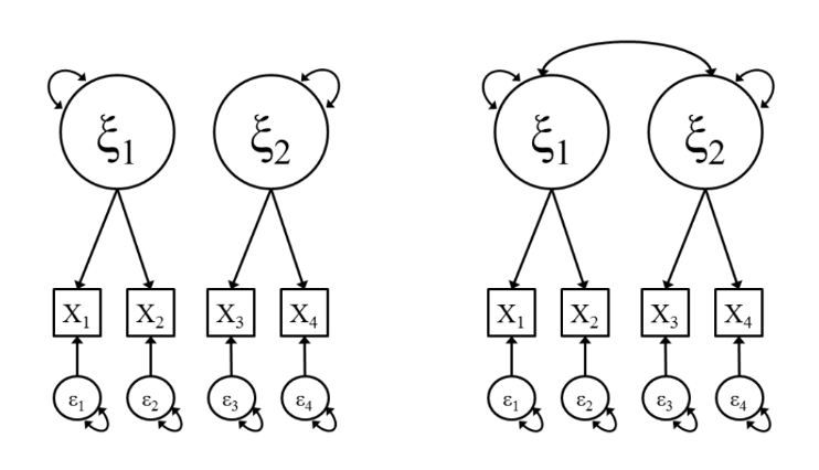
Figure 16.1: Two-factor CFA models with two indicators per factor. Model A (left) has orthogonal (uncorrelated) factors, whereas Model B (right) has correlated factors.
16.1 Empirical check of Model A
Script 16.1 is the script for the two steps to check identification of Model A.
Script 16.1
## STEP 1: calculate the model-implied covariance matrix
LAMBDA <- matrix(c(.8, 0,
                   .7, 0,
                    0,.8,
                    0,.7), nrow = 4, ncol = 2, byrow = TRUE)
PHI <- matrix(c(1, 0,
                    0, 1), nrow = 2, ncol = 2, byrow = TRUE)
THETA <- diag(.5, nrow = 4, ncol = 4)

SIGMA <- LAMBDA %*% PHI %*% t(LAMBDA) + THETA
obsnames <- c("x1","x2","x3","x4")
dimnames(SIGMA) <- list(obsnames, obsnames)
SIGMA

## STEP 2: fit model to the covariance matrix from Step 1
EmpiricalCheck <- '
    # regressions
    Ksi1 =~ L11*x1 + L21*x2
    Ksi2 =~ L32*x3 + L42*x4

    # residual variances
    x1 ~~ TH11*x1
    x2 ~~ TH22*x2
    x3 ~~ TH33*x3
    x4 ~~ TH44*x4

    # (co)variances common factors
    Ksi1 ~~ F11*Ksi1
    Ksi2 ~~ F22*Ksi2
    Ksi1 ~~ F21*Ksi2

    # scaling constraints
    F11 == 1
    F22 == 1
    F21 == 0
'
## fit model
EmpiricalCheckOut <- lavaan(EmpiricalCheck, sample.cov = SIGMA,
        sample.nob = 100, likelihood = "wishart", fixed.x = FALSE)
## compare results to specified parameters
lavInspect(EmpiricalCheckOut, "est")$lambda
LAMBDA
lavInspect(EmpiricalCheckOut, "est")$psi
PHI
lavInspect(EmpiricalCheckOut, "est")$theta
THETA
When we run this model, lavaan may already give a warning21 that it is unable to compute standard errors (which is usually already a sign that there is something may be wrong with your model). Looking at the output, you will notice that the parameter estimates from Step 2 differ from the ones we specified in Step 1. We can thus conclude that this model is not identified.
Recall from Chapter 14 that a factor with only two indicators requires additional constraints to be identified, beyond simply choosing a scale by setting the factor variance or a reference variable’s factor loading to 1. There are only three observed pieces of information about two indicators: two variances and a covariance. Thus, estimating more than three parameters leads to under-identification. So two possible solutions to identify Model A would be (a) to fix both factor loadings to 1 and estimate the factor variance or (b) to fix the factor variance to 1 and constrain the factor loadings to equality. These additional constraints are necessary whenever a two-indicator factor does not have a substantial correlation with another factor in the model.
When the factors in Model B have a correlation that is substantially different from zero, the model actually is identified (Steiger, 2002). This seems counter-intuitive because Model B is specified the same way regardless of the data to which Model B is fit. That is, the covariances among indicators of the different factors provide a unique set of best-fitting estimated model parameters. However, Model B is empirically under-identified when the factor correlation is near zero (i.e., when the indicators from different factors are nearly uncorrelated).
Script 16.2 checks the identification of Model B, assuming a moderate correlation (\(r = .3\)).
Script 16.2
## STEP 1: calculate the model-implied covariance matrix
LAMBDA <- matrix(c(.8, 0,
                   .7, 0,
                    0,.8,
                    0,.7), nrow = 4, ncol = 2, byrow = TRUE)
PHI <- matrix(c( 1, .3,
            .3,  1), nrow = 2, ncol = 2, byrow = TRUE)
THETA <- diag(.5, nrow = 4, ncol = 4)

SIGMA <- LAMBDA %*% PHI %*% t(LAMBDA) + THETA
obsnames <- c("x1","x2","x3","x4")
dimnames(SIGMA) <- list(obsnames, obsnames)
SIGMA

## STEP 2: fit model to the covariance matrix from Step 1
EmpiricalCheck <- '
    # regressions
    Ksi1 =~ L11*x1 + L21*x2
    Ksi2 =~ L32*x3 + L42*x4
    # residual variances
    x1 ~~ TH11*x1
    x2 ~~ TH22*x2
    x3 ~~ TH33*x3
    x4 ~~ TH44*x4
    # (co)variances common factors
    Ksi1 ~~ F11*Ksi1
    Ksi2 ~~ F22*Ksi2
    Ksi1 ~~ F21*Ksi2
    # scaling constraints
    F11 == 1
    F22 == 1
'

## fit model
EmpiricalCheckOut <- lavaan(EmpiricalCheck, sample.cov = SIGMA,
        sample.nob = 100, likelihood = "wishart", fixed.x = FALSE)
## compare results to specified parameters
lavInspect(EmpiricalCheckOut, "est")$lambda
LAMBDA
lavInspect(EmpiricalCheckOut, "est")$psi
PHI
lavInspect(EmpiricalCheckOut, "est")$theta
THETA
If you run this modified script, you will notice that the parameter estimates are exactly equal to our chosen values from Step 1. This is a necessary requirement for identification, but not sufficient. So we only know that the model might be identified, but we cannot be sure whether it really is identified without using algebraic methods. The curious reader can find algebraic proof that Model B is identified in Steiger (2002).
References
Steiger, J. H. (2002). When constraints interact: A caution about reference variables, identification constraints, and scale dependencies in structural equation modeling. Psychological Methods, 7(2), 210–227. doi:10.1037//1082-989X.7.2.210
In version 0.5-22, there is no warning, so the model appears to converge normally. This shows that it is important to conduct an empirical check, because the researcher would not know that this model is not identified.↩︎